Color Ordered Amplitude Coefficients
$\circ\,$ To obtain cross sections we have to compute amplitudes
$$
\require{color}
\require{amsmath}
\hat{σ}_{n}=\frac{1}{2\hat{s}}\int d\Pi_{n-2}\;(2π)^4δ^4\big(\sum_{i=1}^n p_i\big)\;|\overline{\mathcal{A}(p_i,h_i,a_i,μ_F, μ_R)}|^2
$$
$\circ\,$ The gauge group dependence is fairly well understood, through color decompositions
$$
\mathcal{A}(p_i,h_i,a_i,μ_F, μ_R) = \sum_{\sigma} \mathcal{C}(\sigma \circ a_i) \times A(\sigma \circ \{p_i, h_i\}, \mu_F, \mu_R)
$$
$\circ\,$ So we can deal with either color-ordered amplitudes
$$
\mathcal{A}(\lambda^\alpha, \tilde \lambda^{\,\dot\alpha}) = \sum_{\substack{\Gamma,\\ i \in M_\Gamma}} \frac{ \sum_{k=0}^{\text{finite}} \, {\color{red}c^{(k)}_{\,\Gamma, i}}(\lambda^\alpha, \tilde \lambda^{\,\dot\alpha}) \, \epsilon^k}{\prod_j (\epsilon - a_{ij})} \, I_{\Gamma,i}\left( (\lambda\tilde\lambda)^{\alpha\dot\alpha}, \epsilon\right) \;, \;\;\text{with} \quad a_{ij} \in \mathbb{Q}
$$
$\phantom{\circ}\,$ or finite remainders (arguably better since they retain all the physical info)
$$
\mathcal{R}^{(\ell-loop)} = \mathcal{A}^{(\ell)}_R - \sum_{i=1}^{\ell} I^{(\ell-i)} \mathcal{A}^{(i-1)} + \mathcal{O}(\epsilon) = \sum_i {\color{red}{r_{i}(\lambda,\tilde\lambda)}} \, h_i(\lambda\tilde\lambda)
$$
Number of Indep. Functions w/o Subtraction
Numerical Generalized Unitarity
Ita (‘15)
Abreu, Febres Cordero, Ita, Page, Zeng (‘17)
$\circ$ We have an Ansatz for the loop integrand
$$
\require{color}
\displaystyle A(\lambda, \tilde\lambda, \ell) = \sum_{\Gamma} \, \sum_{i \in M_\Gamma \cup S_\Gamma} \, c_{\,\Gamma,i}(\lambda, \tilde\lambda) \, \frac{m_{\Gamma,i}(\lambda\tilde\lambda, \ell)}{\textstyle \prod_{j} \rho_{\,\Gamma,j}(\lambda\tilde\lambda, \ell)}
$$
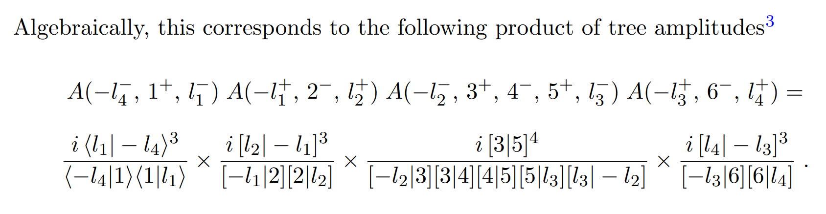
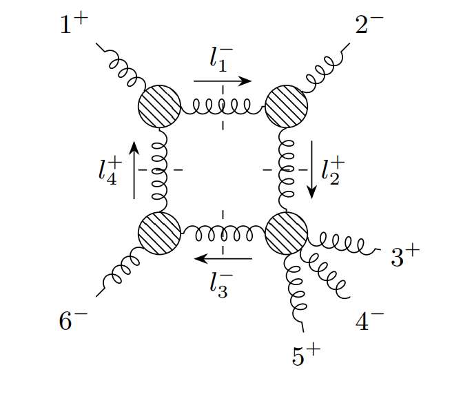
$\circ$ Generalized unitarity relates cuts of loop amplitudes to products of trees
$$
\require{color}
\displaystyle \sum_{\text{states}} \, \prod_{\text{trees}} A^{\text{tree}}(\lambda, \tilde\lambda, \ell)\big|_{\text{cut}_{\Gamma}} = \sum_{\substack{\Gamma' \ge \Gamma, \\ i \in M_\Gamma' \cup S_\Gamma'}} \kern-2mm c_{\,\Gamma',i}(\lambda, \tilde\lambda) \, \frac{m_{\Gamma',i}(\lambda\tilde\lambda, \ell)}{\displaystyle \prod_{j\in P_{\Gamma'} / P_{\Gamma}} \rho_{j}(\lambda\tilde\lambda, \ell)}\Bigg|_{\text{cut}_\Gamma}
$$
Numerical Berends-Giele recursion for LHS, solve for coeffs. in RHS.
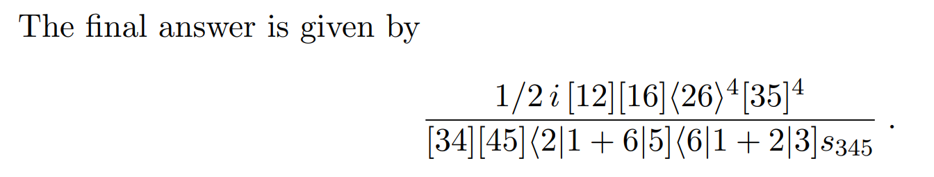
Six-Gluon Box Example in D=4
Integration By Parts Reduction
$\circ$ Master / surface decomposition for non-planar topologies
$$
\require{color}
\begin{align}
\kern-25mm \text{IBP-generating vectors: } & \quad \displaystyle \int d^D \ell \frac{\partial }{\partial \ell^\mu_a} \frac{v^\mu_a(\ell)}{\rho_1 \dots \rho_N} = 0 \quad (\text{in dim. reg.}) \\[2mm]
\kern-25mm \text{No propagator doubling: } & \quad \displaystyle \sum_{a, \mu} v^\mu_a(\ell) \frac{\partial \rho_i}{\partial \ell^\mu_a} - f_i(\ell)\rho_i = 0
\end{align}
$$
$(v^\mu_a, f_i)$ form a syzygy module, solved for in embedding space using Singular + linear algebra.
$\circ$ Semi-numerical surface terms: $\quad m_{i\in S_\Gamma}(\ell \leftarrow \text{analytical}, s_{ij} \leftarrow \text{numerical})$
$\kern20mm\star$ dependance on external kinematics ($s_{ij}$) obtained from sparse linear systems.
$\circ$ Little group information retained throughout the computation
$\kern20mm\star$ genuine $c_{\Gamma,i}(\lambda, \tilde\lambda)$ instead of $c_{\Gamma,i}(\lambda\tilde\lambda)$ + conventions for the polarization states.
Complexity Swell of Amplitudes Coefficients
$\circ\,$ The rational coefficients take the form
$$
\displaystyle r(|i\rangle,[i|) = \frac{\mathcal{N}(|i\rangle,[i|)}{\prod_j \mathcal{D}_j^{q_{ij}}(|i\rangle,[i|)}
$$
$\phantom{\circ}\,$ with $\mathcal{N}$ and $\mathcal{D}$ polynomials of spinor brackets.
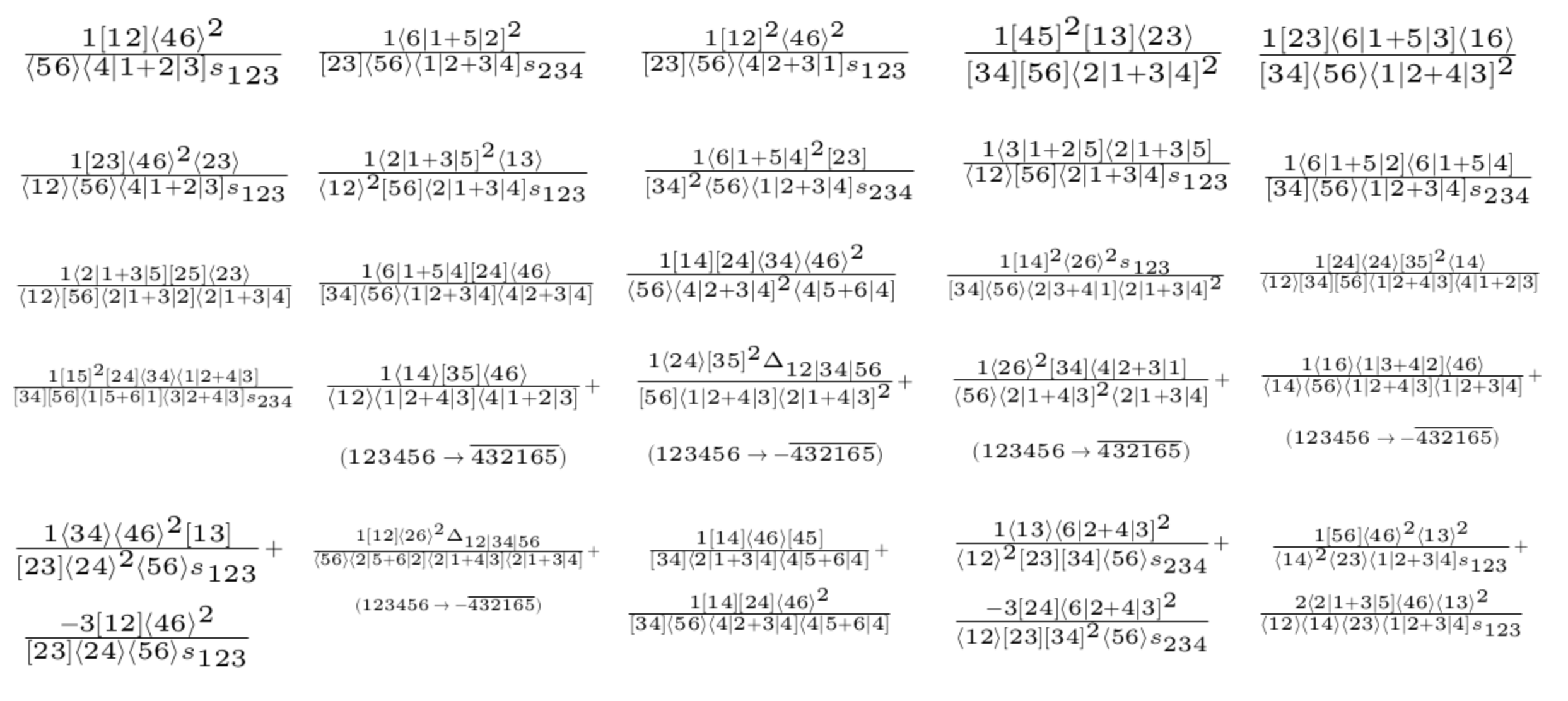
$\circ\,$ For example, consider this 2-loop $Vjj$ coefficient
($s_{56}=p^2_V$ is a zero, $⟨3|1+4|2]^{5}Δ_{23|14|p_V}^{4}$ are poles):
GDL, Ita, Page, Sotnikov (W.I.P.)
Abreu, Febres Cordero, Ita, Klinkert, Page, Sotnikov ('21),$\quad$
$$
r^{(73 \text{ of } 120)}_{\bar{u}^+g^-g^+d^-(V\rightarrow \ell^+ \ell^-)} = \frac{105}{128}\frac{⟨2|1+4|3]⟨4|2+3|1]⟨6|1+4|5]s_{14}s_{23}s_{56}(s_{124}-s_{134})(s_{123}-s_{234})(s_{25}+s_{26}+s_{35}+s_{36})}{\color{orange}{⟨3|1+4|2]}\color{red}{Δ_{23|14|56}^4}} + \\
\Bigg[6\frac{[12]^2⟨13⟩[25]⟨34⟩⟨36⟩s_{56}(s_{124}-s_{134})}{\color{orange}{⟨3|1+4|2]^5}}\Bigg] + \Bigg[ \; \Bigg]_{1234\rightarrow \overline{4321}}+ \mathcal{O}\left(\frac{1}{⟨3|1+4|2]^{4}Δ_{23|14|56}^{3}}\right)
$$
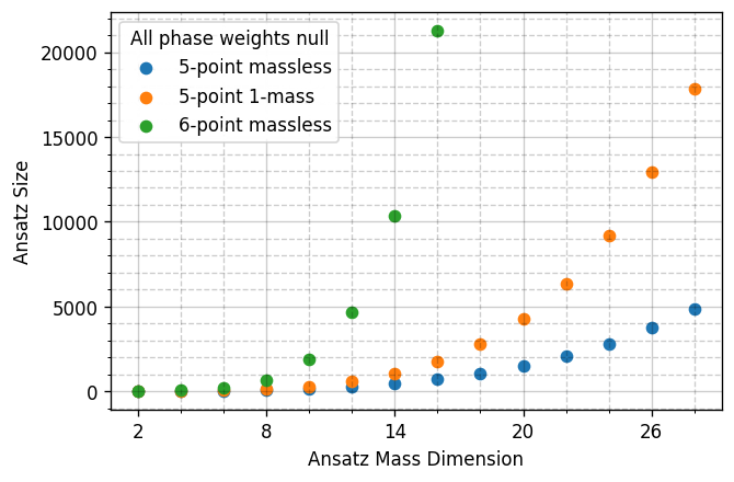
$\circ\,$ The first fraction has Ansatz(mass dimension: 16, phase weights: [-1, 1, -1, 1, -1, 1]) of size:
$$
16488 {\small\text{ (six-point massless) }} \rightarrow 4200 {\small \text{ (five-point one-mass) }} \rightarrow 2429 {\small \; (Δ_{23|14|56}-\text{residue})} \rightarrow 1 \; \small{(??)}
$$
Plan for this talk
$1.\,$ Rational Functions w/ Constraints: Algebra and Geometry
$2.\,$ External and Internal Masses
$3.\,$ Vector Spaces over Fields of Fractions
$4.\,$ Analytic Reconstruction
Polynomials ‘‘Modulo Equivalence Relations’’
$\circ$ The most obvious equivalence relation we need to deal with is momentum conservation
$$
q, r: \text{ polynomials }, \qquad q \sim r \quad \text{if} \quad q - r \propto \sum_i p_i = \sum_i |i⟩[i| = 0
$$
$\circ$ Then we have Schouten identities, e.g.
$$
\langle j|k\rangle \langle l|i\rangle + \langle k|i\rangle \langle l|j\rangle + \langle i|j \rangle \langle l|k\rangle = 0
$$
$\circ$ Note that this happens whenever we have (enough) vectors in the game!
$$
\text{tr}_5(2345)p^µ_1 - \text{tr}_5(1345)p^µ_2 + \text{tr}_5(1245) p^µ_3 - \text{tr}_5(1235)p^µ_4 + \text{tr}_5(1234)p^µ_5 = 0
$$
$\circ$ One more distinct example later ... with masses!
Polynomial Quotient Rings
$\circ$ Without equivalences, we would have a polynomial ring
$$\displaystyle \kern-50mm S_n = \mathbb{F}\left[|1⟩, [1|, \dots, |n⟩, [n|\right]$$
$\phantom{\circ}$ the field $\mathbb{F}$ can be any of $\mathbb{Q},\mathbb{R},\mathbb{C},\mathbb{F}_p,\mathbb{Q}_p,\dots$
$\circ$ Equivalence relations define ideals, e.g.
$$
\displaystyle J_{\Lambda_n} = \Big\langle \sum_i |i⟩[i| \Big\rangle_{S_n}
$$
Artist's Impression of $V(J_{\Lambda_n})$
I can't draw in $4n$ dims!
$\phantom{\circ}$ Wwo polynomials $q$ and $r$ are equivalent if $q-r\in J_{\Lambda_n}$
$\circ$ What we need is a polynomial quotient ring$\kern-4mm\phantom{x}^{\star}$: $\;R_n = S_n / J_{\Lambda_n} $
$r_i(\lambda, \tilde\lambda)$ at $n$-point belong to the Field of Fractions$\kern-4mm\phantom{x}^{\dagger}$ of $R_n$
$\kern-4mm\phantom{x}^\star R_4$ is "weird" (not a UFD), but it proves that polynomial rings are insufficient;
$\;\kern-4mm\phantom{x}^\dagger$ The field of fractions of $R_3$ does not exist.
Singularities of Amplitudes
$\circ$ Let us consider a very simple example (at 4-point)
$\displaystyle \kern-50mm iA_{g^-g^-g^+g^+}^{\text{tree}} = \frac{\langle 12 \rangle^3}{\langle 23 \rangle \langle 34 \rangle \langle 41 \rangle} = \frac{[34]^3}{[12][23][41]} $
$\phantom{\circ}$ is, say, $\langle 23 \rangle$ a pole of this amplitude?
Artist's Impression of $V(\big\langle \langle 23 \rangle\big\rangle_{R_4})$
as the union of two irreducibles
$\circ$ The question is ill posed! Let's consider it geometrically.
$\phantom{\circ} \langle 23 \rangle$ does not identify an irreducible variety in $R_4$.
$\phantom{\circ}$ Algebraically, we can compute primary decompositions , e.g.
$\displaystyle \big\langle \langle 23\rangle \big\rangle_{R_4} = {\color{orange} \big\langle \langle 23\rangle, [14] \big\rangle_{R_4}} \cap {\color{blue} \big\langle \langle 12\rangle, \langle 13 \rangle, \langle 14\rangle, \langle 23\rangle, \langle 24 \rangle, \langle 34 \rangle \big\rangle_{R_4}} $
$\phantom{\circ}$ On the first branch there is a simple pole, on the latter branch the amplitude is regular.
Poles & Zeros $\;\Leftrightarrow\;$ Irreducible Varieties $\;\Leftrightarrow\;$ Prime Ideals
Physics $\kern38mm$ Geometry $\kern38mm$ Algebra
Spinor Alphabets
$1.$ little group covariant LCD (less spurious poles); $\;\;2.$ avoiding parity even/odd split.
$\Rightarrow\;$ fewer and simpler functions to reconstruct compared to Mandelstams or Twistors.
$\circ\,$ The denominator factors $\mathcal{D}_j$ are conjectured to be restricted to the letters of the symbol alphabet
Abreu, Dormans, Febres Cordero, Ita, Page ('18)
$$
\displaystyle \{\mathcal{D}_{\{1,\dots,35\}}\} = \bigcup_{\sigma \; \in \; \text{Aut}(R_5)} \sigma \circ \big\{ \langle 12 \rangle, \langle 1|2+3|1] \big\} \, , \qquad \text{Aut}(R_5) = \mathcal{P} \times \mathcal{S}_5
$$
$\small\qquad\color{green}\text{Identical to 1-loop!}$
$\circ\,$ Beyond 5-point things get tough
$\displaystyle \kern-10mm \{\mathcal{D}_j\} = \bigcup_{\sigma \; \in \; \text{Aut}(R_6)} \sigma \circ \big\{ \langle 12 \rangle, \langle 1|2+3|1], \langle 1|2+3|4], s_{123}, \Delta_{12|34|56}, ⟨3|2|5+6|4|3]-⟨2|1|5+6|4|2] \big\} $
$\small\qquad\color{red}\text{New @ 2-loop planar!}\qquad$
$$
\displaystyle \kern-10mm \{\mathcal{D}_j\} = \bigcup_{\sigma \; \in \; \text{Aut}(R_7)} \sigma \circ \big\{ \langle 12 \rangle, \langle 1|2+3|1], \langle 1|2+3|4], s_{123}, \Delta_{123|45|67},
$$
$$
\kern130mm\langle1|2+3|4+5|1\rangle, \langle1|3+4|5+6|2\rangle , \dots(?)\big\}
$$
$\phantom{\circ}$ Non-trivial statement (not proven!): all irreducible polynomials generate prime ideals in $R_{m>4}$.
Least Common Denominator
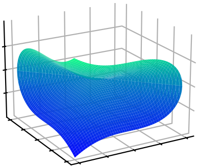
$\circ\,$ Can't draw pictures in high (complex) dimensions, so let's consider the simplified case $\mathbb{R}[x, y, z]$.
$\circ\,$ Say we have a potential denominator factor $\mathcal{D} = xy^2 + y^3 - z^2$
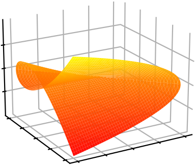
${\color{orange}\mathcal{D} = (xy^2 + y^3 - z^2)}$
A function $f_i(x,y,z)$ may or may not have $\mathcal{D}$ as a pole, depending on what happens on $V(\langle\mathcal{D}\rangle)$
$\displaystyle \lim_{\mathcal{D}_j \rightarrow \epsilon} f_i(x,y,z) \sim \frac{1}{\epsilon^{q_{ij}}} $
$q_{ij}$ is the order of the pole ($\mathbb{Z}^+$) or zero ($\mathbb{Z}^-$).
The LCD tells us about what happens on surfaces with one less dimension than the full space.
Codimension-One Slices
$\circ\,$ What we have reliably available at 2-loop are $\mathbb{F}_p$ evaluations.
$\phantom{\circ}\,$ ($\mathbb{Q}_p$ is doable, but potentially very slow / unstable - dependening on the point.)
$\circ\,$ Issue: the limit can be taken in $\mathbb{R}$, $\mathbb{C}$, $\mathbb{Q}_p$ but ${\color{red}\text{not}}$ in $\mathbb{F}_p$ .
$\circ\,$ Solution: univariate Thiele rational interpolation on a line going through each $V(\langle \mathcal{D}_j \rangle)$
$$
\displaystyle |i\rangle \rightarrow |i\rangle (t) = |i\rangle + t c_i |\eta\rangle , \qquad |i] \rightarrow |i] \, , \qquad
\text{s.t.} \quad \sum_i c_i |i] = 0
$$
$\circ\,$ After interpolation on the (anti-)holomorphic slice, the rational functions read
$$
\displaystyle r_i(t) = \frac{\mathcal{N}(t)}{\prod_j (t-t_{\mathcal{D}_j})^{q_{ij}}}
$$
$\phantom{\circ}\,$ where $t_{\mathcal{D}_j}$ is simply the solution to $\mathcal{D}_j(t) = 0$. We read off the $q_{ij}$.
$\circ\,$ Issue: in $\color{red}\text{LCD}$ form the Ansatz has $\color{red}\text{too many free parameters}$, e.g. $\bar{u}^+g^+g^+d^-(V\rightarrow \ell^+ \ell^-)$
size(Ansatz(54, [0, 0, 2, 2, -1, 1])) = $1\,209\,546$
Multivariate Partial Fractions
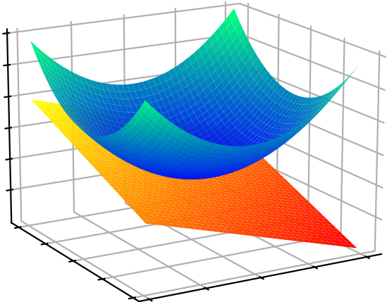
$\circ\,$ To distinguish $\displaystyle \frac{\mathcal{N}_{12}}{W_1W_2}$ from $\displaystyle \frac{\mathcal{N}_1}{W_1} + \frac{\mathcal{N}_2}{W_2}$, look at $W_1 \sim W_2 \rightarrow \epsilon \ll 1$. Geometrically:
${\color{orange}V(W_1) = V(\langle xy^2 + y^3 - z^2 \rangle)}$
${\color{blue}V(W_2) = V(\langle x^3 + y^3 - z^2\rangle )}$
$V(W_1) \cap V(W_2)$
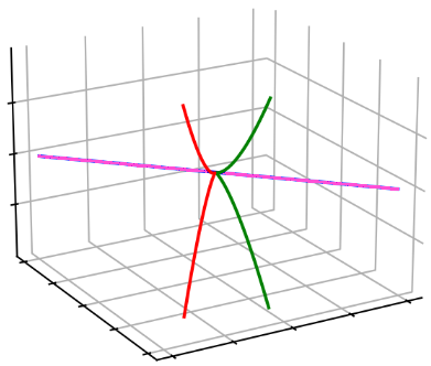
$\circ\,$ Primary decompositions of sets of polynomials ( ideals ), anogous to integers:
$60 = 5 \times 3 \times 2^2$
$\langle{\color{orange}xy^2 + y^3 - z^2}, {\color{blue}x^3 + y^3 - z^2}\rangle = \\
{\color{magenta}\langle z^2,x+y\rangle} \cup {\color{green}\langle y^3-z^2,x\rangle} \cup {\color{red}\langle2y^3-z^2,x-y\rangle}$
$\circ\,$ Whether a partial fraction decomposition is possible depends on the behavior on the 3 lines.
Beyond Partial Fractions
$\circ$ $\color{red}\text{Case 0}$: the ideal does $\color{green}\text{not involve denominator factors}$.
E.g. a 6-point function $c_i$ has a pole at $⟨1|2+3|4]$ but not at $⟨4|2+3|1]$,
yet it is regular on the irreducible surface $V(\big\langle ⟨1|2+3|4], ⟨4|2+3|1] \big\rangle)$. Then
$\displaystyle c_i \sim \frac{⟨4|2+3|1]}{⟨1|2+3|4]} + \mathcal{O}(⟨1|2+3|4]^0) \; \text{ instead of } \; c_i \sim \frac{1}{⟨1|2+3|4]} + \mathcal{O}(⟨1|2+3|4]^0)$
$\circ$ $\color{red}\text{Case 1}$: the $\color{green}\text{degree of vanishing is non-uniform}$ across branches, for example:
$\displaystyle \frac{s_{14}-s_{23}}{⟨1|3+4|2]⟨3|1+2|4]}$
has a double pole on the first branch, and a simple pole on the second branch of
$\big\langle⟨1|3+4|2], ⟨3|1+2|4]\big\rangle_{R_6} = \big\langle ⟨13⟩, [24] \big\rangle_{R_6} \cap \big\langle ⟨1|3+4|2], ⟨3|1+2|4], (s_{14}-s_{23})\big\rangle_{R_6}$
$\circ$ $\color{red}\text{Case 2}$: ideal is $\color{green}\text{non-radical}$
$\displaystyle \small \kern0mm \sqrt{\big\langle {\color{black}⟨3|1+4|2]}, {\color{black}Δ_{23|14|56}} \big\rangle_{R_6}} = \big\langle {\color{black}⟨3|1+4|2]}, {\color{black}s_{124}-s_{134}} \big\rangle_{R_6} $
External Masses
$\circ\,$ Rescale propagators to make them look massless, e.g.
$$
\mathcal{A}(pp \rightarrow Vjj) = \frac{p_V^2}{p_V^2-m_V^2}\mathcal{A}(pp \rightarrow Vjj)\Big|_{m_V=0}
$$
$\circ\,$ Say $p_V^2 = \langle56\rangle[65]$, we observe $\mathcal{N}_i \in \Big\langle \langle56\rangle , [56] \Big\rangle$ for all 2-loop coeffs. in $pp\rightarrow Vjj$.
$\circ\,$ In general, the singularities of amplitudes w/ massess look like those in the decay kinematics
$$
\text{e.g.:} \qquad \{1,2,3,\boldsymbol{4},\boldsymbol{5}\} \sim \{1,2,3,(\boldsymbol{4}\rightarrow4+5),(\boldsymbol{5}\rightarrow6+7)\} + \text{constraints (e.g. deg. bound.)}
$$
Modifying the Quotient Ring
$\circ\,$ $pp\rightarrow hhj$ with exact $m_{top}$ dependence at LO/1-loop, subject to $p_{h_1}^2 = p_{h_2}^2$.
$\phantom{\circ}\,$ We work in the modified version of the $R_7$ q-ring, namely:
$$
\tilde{R}_7 = \mathbb{Q}_p\Big[ |1\rangle, [1|, \dots, |7\rangle, [7| \Big] \big/ \Big\langle \sum_{i=1}^7 |i\rangle[i|, s_{45} - s_{67} \Big\rangle
$$
Internal Masses - The Easy Case
$\circ\,$ If the only dependence is in the numerator, then a Taylor expansion is generally enough (like $\epsilon$).
$\phantom{\circ}\,$ For instance, taking results from $0 \rightarrow q\bar q (V\rightarrow \ell\bar\ell )(V'\rightarrow \ell'\bar\ell') g$ w/ massive q-loop
$$
\begin{eqnarray} \label{basicexpansion}
d_{\{i\times j\times k\}}&=\;(v_L^2+v_R^2)\, &\big[m^0 d_{\{i\times j\times k\}}^{(0)}+m^2 d_{\{i\times j\times k\}}^{(2)}+m^4 d_{\{i\times j\times k\}}^{(4)}\big] \nonumber \\
&\;+\;v_L v_R &\big[ m^2 \tilde{d}_{\{i\times j\times k\}}^{(2)}+m^4 \tilde{d}_{\{i\times j\times k\}}^{(4)} \big] \, .
\end{eqnarray}
$$
$\circ\,$ Where e.g. $d_{\{12\times34\times56\}}^{(4)}$ is: (using $\Gamma_{34|56} = |3+4|5+6|$, and tilde for anti-symm.)
$$
d_{\{12\times34\times56\}}^{(4)}=\frac{[2|\tilde\Gamma_{34|12|56}|1\rangle}
{s_{12}s_{34}s_{56}\langle7|\Gamma_{34|56}|7\rangle}
\left(\frac{[4|\tilde\Gamma_{34|12|56}|3\rangle[6|\tilde\Gamma_{34|12|56}|5\rangle}
{\langle7|\Gamma_{34|56}|7\rangle[7|\Gamma_{34|56}|7]}
-\langle3|5\rangle[4|6]
\right)
$$
$\circ\,$ Which follows from the following primary decomposition
$$
\big\langle ⟨7|\Gamma_{34|56}|7⟩, [7|\Gamma_{34|56}|7] \big\rangle = \big\langle ⟨7|\Gamma_{34}|7], ⟨7|\Gamma_{56}|7], ⟨7|\Gamma_{34|56}|7⟩, [7|\Gamma_{34|56}|7] \big\rangle \nonumber \\
\kern50mm \quad \cap \; \big\langle ⟨7|\Gamma_{34|56}|7⟩, [7|\Gamma_{34|56}|7], \tilde\Gamma_{12|34|56} \big\rangle \, .
$$
Internal Masses - The Hard Case
$\circ\,$ The poles have mixed mass-kinematics dependence, e.g.
$$
(-s_{12}⟨1|\boldsymbol{5}|\boldsymbol{4}|3⟩[32]⟨23⟩[3|\boldsymbol{4}|\boldsymbol{5}|1]+m_t^2([1|2|3|\boldsymbol{4}|1⟩-⟨1|2|3|\boldsymbol{4}|1])^2) \\
(-s_{13}⟨1|\boldsymbol{4}|2]⟨2|\boldsymbol{4}|1]⟨2|\boldsymbol{5}|3]⟨3|\boldsymbol{5}|2]+m_t^2([1|2|3|\boldsymbol{4}|1⟩-⟨1|2|3|\boldsymbol{4}|1])^2)
$$
$\phantom{\circ}\,$ For instance, this happens at one loop with $D=4$ cuts and pentagon diagrams.
$\circ\,$ The "proper" approach would probably be to add $m_t$ to the q-ring and compute decompositions.
$\phantom{\circ}\,$ This is highly non-trivial; also hard to avoid spurious singularities, e.g. $\text{tr}_5$ or spurious $\langle ij\rangle$.
$\circ\,$ An approach is to use effective pentagon coeffs., schematically
$$
\text{Box} = (\text{Reduction coeff.})\times(\text{Effective pentagon}) + (\text{Effective Box})
$$
$\phantom{\circ}\,$ where only the Effective pentagon has the $m$-dependent pole.
$\circ\,$ (Discussion) When does this happen at 2-loop? Do you need 9 propagators?
Vector Spaces
of Rational Functions
GDL, Ita, Page, Sotnikov - to appear; $\quad$
GDL, Ita, Klinkert, Sotnikov
arXiv:2311.10086
Complexity of the Reconstruction
$\circ\,$ Sort the $r_i$ by mass dimension of $\mathcal{N}$ ($\approx$ Ansatz size), pick simplest subset forming a basis $r_{i \in \mathcal{B}}$
Picking a Basis
$\circ\,$ We start from something of the form:
$$
R = r_{i\in \mathcal{B}} M_{ij} h_j \, , \qquad M_{ij} \in \mathbb{Q}
$$
$\phantom{\circ}\,$ with $r_{i\in \mathcal{B}} \subset r_i$, i.e. $M_{ij}$ is in reduced row echelon form, up to a permutation of columns.
$\circ\,$ Basic idea: change basis from a subset of pentagon function coefficients, to linear combinations
$$
\tilde{r}_{i'} = O_{i'i} \, r_{i \in \mathcal{B}} \quad \text{s.t.} \quad \text{rank}(O_{i'i}) = \text{dim(span}_{FF(R_5), \mathbb{Q}}(r_{i}))
$$
$\circ\,$ Key insight:
$$
\text{dim(span}_{FF(R_5), \mathbb{Q}}\left(\lim_{\mathcal{D_j} \rightarrow 0 }r_{i}\right)) \leq \text{dim(span}_{FF(R_5), \mathbb{Q}}(r_{i}))
$$
$\phantom{\circ}\,$ I.e., the pole residues are correlated, build linear combinations that ''remove the overlap''
Correlation of Residues
$\circ\,$ Build Laurent expansions around $t_{\mathcal{D}_k}$
(use same kind of slice as before)
$$
r_{i \in \mathcal{B}} = \sum_{m = 1}^{q_k = \text{max}_i(q_{ik})} \frac{e^k_{im}}{(t-t_{\mathcal{D}_k})^m} + \mathcal{O}((t-t_{\mathcal{D}_k})^0)
$$
$\phantom{\circ}\,$ strictly formal over $\mathbb{F}_p$, but convergent over $\mathbb{Q}_p$ for $(t-t_{\mathcal{D}_k}) \propto p$
$\circ\,$ Repeat for several (anti-)holomorphic slices, build vectors
$$
\vec{e}^k_{im} = (e^k_m)_{ij} = \{ e^k_{im}(\text{slice}_1), \dots, e^k_{im}(\text{slice}_n) \}
$$
$\circ\,$ By Gaussian elimination on the matrix $(e^k_m)_{ij}$ we can partition the space:
$$
\text{span}_{\vec{\mathbb{Q}},\mathbb{Q}}(r_{i \in \mathcal{B}}) = \text{column}_{\vec{\mathbb{Q}},\mathbb{Q}}(\text{Res}(r_{i \in \mathcal{B}}, \mathcal{D}_k^m)) \oplus \text{null}_{\vec{\mathbb{Q}},\mathbb{Q}}(\text{Res}(r_{i \in \mathcal{B}}, \mathcal{D}_k^m))
$$
Interpretation of $\text{null}_{\vec{\mathbb{Q}},\mathbb{Q}}(\text{Res}(r_{i \in \mathcal{B}}, D_k^m)) \cdot r_{i \in \mathcal{B}}$: functions that do not have a $D_k^m$ singularity
Breadth-First Search
$\circ\,$ If a function $\tilde{r}$ does not have poles $D_{k_1}^{m_1}$ and $D_{k_2}^{m_2}$, then
$$
\tilde{r} \in \text{span}_{FF(R_5),\mathbb{Q}}\Bigg[\Big(\text{null}_{\vec{\mathbb{Q}},\mathbb{Q}}(\text{Res}(r_{i \in \mathcal{B}}, D_{k_1}^{m_1})) \cap \text{null}_{\vec{\mathbb{Q}},\mathbb{Q}}(\text{Res}(r_{i \in \mathcal{B}}, D_{k_2}^{m_2}))\Big)_{i'i} \; \cdot \; r_{i\in \mathcal{B}}\Bigg]
$$
$\circ\,$ Build linear combination that remove as many singularities as possible, without dropping rank
$$
\displaystyle O_{i'i} = \cap_{k, m} \, \text{nulls}_{\vec{\mathbb{Q}},\mathbb{Q}} \qquad \text{(schematically)}
$$
$\circ\,$ This is done by searching a tree of possibilities of which pole gets dropped to which order.
$\phantom{\circ}\,$ Several optimizations required to search an otherwise proibitively large space, naively of size
$$
\prod_k (m_k + 1) \quad \text{with } \; k \;\text{ enumerating } \; D_k^{m_k}
$$
Least Least-Common-Denominator
$\circ$ In other words, we have reshuffled the $r_i$ by linear combinations of the others $r_{j\neq i}$
$\displaystyle \tilde{r}_i = \sum_{j\neq i} O_{ij} r_j + r_i$
$\circ\,$ The rational functions now take the form
$$
\displaystyle \tilde{r}_i(|i\rangle,[i|) = \frac{\tilde{\mathcal{N}}(|i\rangle,[i|)}{\prod_j D_j^{\tilde{q}_{ij}}(|i\rangle,[i|)}
$$
$\phantom{\circ}\,$ where we have minimized $\sum_j \tilde{q}_{ij}$, compared to the $r_i$.
$\circ\,$ This is the closest thing that I am aware of to a Gram–Schmidt procedure for vector spaces over fields that are not number fields, but in this case fields of fractions over polynomial quotient rings.
$\circ\,$ Can we think of this as defining an inner product on the space of rational functions?
$$
O_{ij} \sim \langle r_i | r_j \rangle \qquad \text{(very schematically)}
$$
(Discussion) Is there a connection to intersection theory?
The Numerator Ansatz
$\circ\,$ The numerator Ansatz takes the form
GDL, Maître ('19)
$\displaystyle \text{Num. poly}(\lambda, \tilde\lambda) = \sum_{\vec \alpha, \vec \beta} c_{(\vec\alpha,\vec\beta)} \prod_{j=1}^n\prod_{i=1}^{j-1} \langle ij\rangle^{\alpha_{ij}} [ij]^{\beta_{ij}}$
$\phantom{\circ}$ subject to constraints on $\vec\alpha,\vec\beta$ due to: 1) mass dimension; 2) little group; 3) linear independence.
$\circ\,$ Construct the Ansatz via the algorithm from Section 2.2 of
GDL, Page ('22)
Linear independence = irreducibility by the Gröbner basis of a specific ideal.
$\circ\,$ Efficient implementation using open-source software only
$\circ\,$ Linear systems solved w/ CUDA over $\mathbb{F}_{2^{31}-1}$ ($t_{\text{solving}} \ll t_{\text{sampling}}$) w/
linac (coming soon-ish)
Some Public Computational Tools
Five-Parton Results in Full Color
GDL, Ita, Klinkert, Sotnikov ('23),
GDL, Ita, Sotnikov ('23);
see also
Agarwal, Buccioni, Devoto, Gambuti, von Manteuffel, Tancredi ('23)
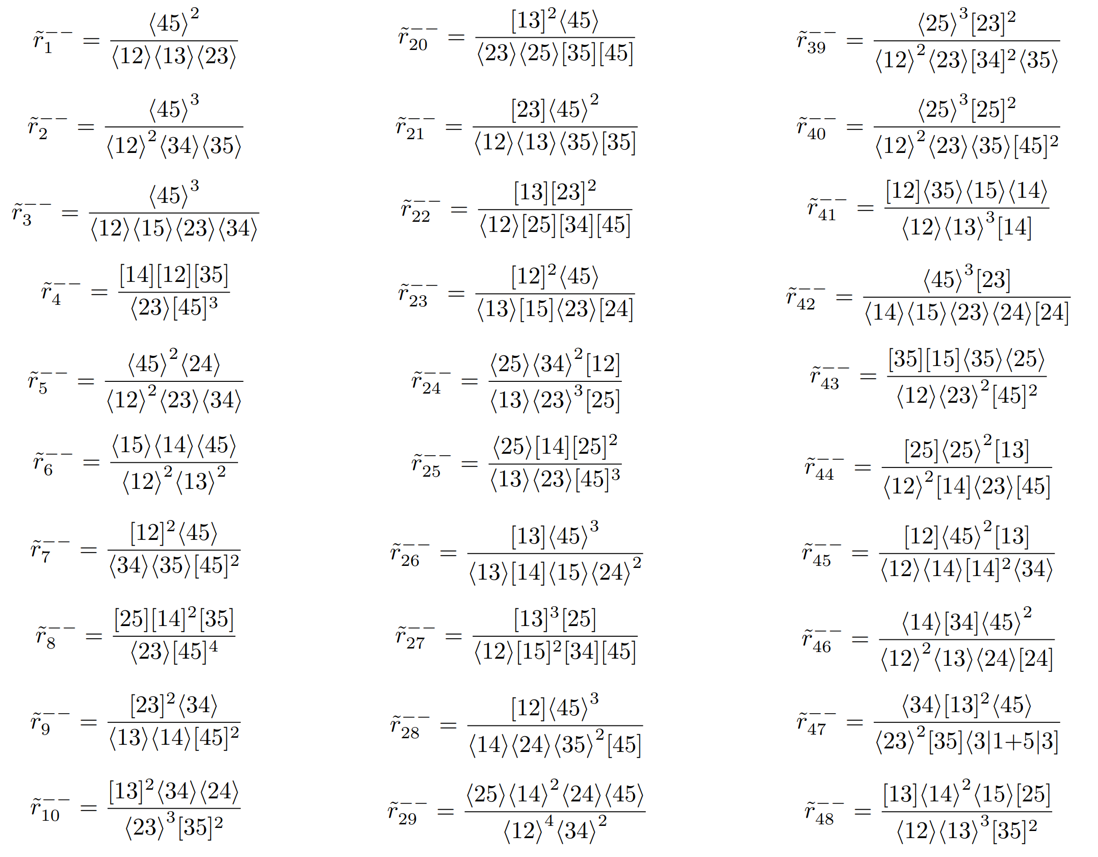
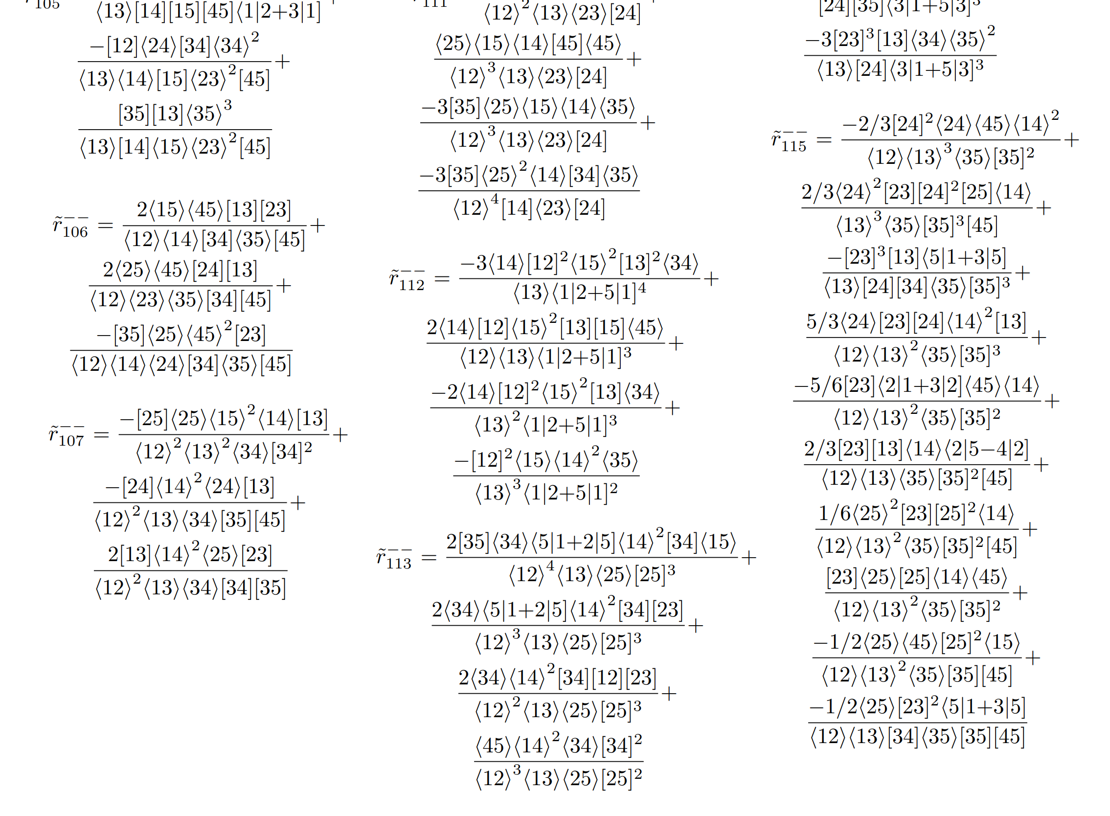
$\circ\,$ The basis of the vector space is now quite easy! ($r_{115}^{--}$ is the most complicated function)
Outlook: More Legs and/or Masses
$\circ\,$ New mathematical tools help tackle the increasing complexity of amplitudes in the precision era.
$\circ\,$ Preliminary results for $pp\rightarrow Wjj$ are around $25 MB$ (down from $1.2GB$ ),
$\phantom{\circ}\,$ with the quark-channel basis functions down to $125 KB$, of which 25 of 92 functions are:
Summary
We talked about:
$1.\,$ Rational Functions in the Field of Fractions of Polynomial Quotient Rings:
$\qquad\circ\,$ How to enforce constraints on polynomials;
$\qquad\circ\,$ The relation between physics $\leftrightarrow$ algebra $\leftrightarrow$ geomtry;
$\qquad\circ\,$ The role of the Least Common Denominator, and how to obtain it
$\qquad\circ\,$ Partial fraction decompositions from higher-codimension information
$2.\,$ Different cases where masses appear:
$\qquad\circ\,$ External masses
$\qquad\circ\,$ Internal masses (simple Laurent expansion)
$\qquad\circ\,$ Internal masses (mass- and kinematic-dependent poles)
$3.\,$ Vector Spaces over Fields of Fractions
$\qquad\circ\,$ Correlation between residues, a.k.a. basis change;
$\qquad\circ\,$ Its consequences on what functions need to be obtained.
$4.\,$ Analytic Reconstructions from an Ansatz