Modern Methods for the Computation of Scattering Amplitudes


Giuseppe De Laurentis

LTP Seminar

Find these slides at gdelaurentis.github.io/slides/psi-ltp-seminar

Introduction

Amplitudes and Cross Sections
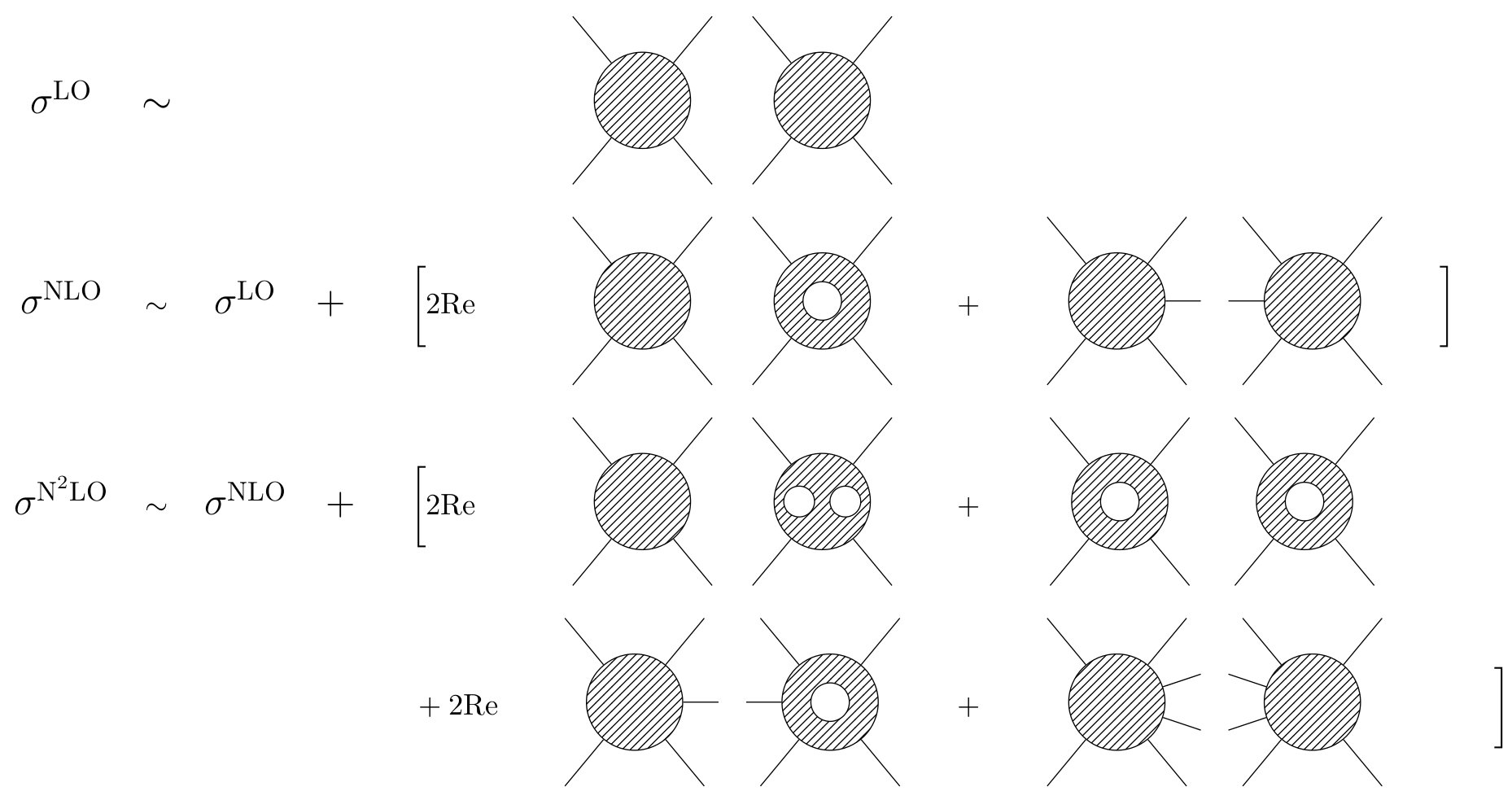
Amplitudes are a key element for computing cross sections. At hadron colliders, we have: $$ \displaystyle σ_{2 \rightarrow n - 2} = \sum_{a,b} ∫ dx_a dx_b f_{a/h_1}(x_a, μ_F) \, f_{b/h_2}(x_b, μ_F) \;\hat{σ}_{ab→n-2}(x_a, x_b, μ_F, μ_R) \\[2mm] \displaystyle \hat{σ}_{n}=\frac{1}{2\hat{s}}\int d\text{LIPS}\;(2π)^4δ^4\big(\sum_{i=1}^n p_i\big)\;|\overline{\mathcal{A}(p_i,\lambda_i,a_i,μ_F, μ_R)}|^2 $$
$$\mathcal{A}_{pp\rightarrow h \rightarrow \gamma\gamma} \sim \frac{1}{m_{\gamma\gamma}^2 - m^2_h + i m_h \Gamma_h}$$ $$\Rightarrow\; \text{Breit–Wigner distribution}$$

Perturbation Theory

$$\displaystyle \mathcal{A}_n / \alpha_s^k = \mathcal{A}_n^{\text{tree}} + \underbrace{\left(\frac{\alpha_s}{2\pi}\right) \mathcal{A}_n^{1-\text{loop}}}_{\sim 10\%} + \underbrace{\left(\frac{\alpha_s}{2\pi}\right)^2 \mathcal{A}_n^{2-\text{loop}}}_{\sim 1\%}$$

Better predictions require both more loops and higher multiplicity.

Processes with additional soft or collinear radiation are indistinguishable from the Born.
State-of-the-Art
$\circ\,$ Focus on all-gluon scattering, as a representative example.

$\mathcal{A}_{n-gluons}^{\ell-loops}$
multiplicity $(n)$
4 5 6 7 8
loops ($\ell$)
0
1
2
3
$\circ\,$Three-loop four-point (analytic)
Caola, Chakraborty, Gambuti, von Manteuffel, Tancredi ('21)
$\circ\,$Two-loop five-point (analytic)
  (Leading Color)
Abreu, Dormans, Febres Cordero, Ita, Page ('18)
$\circ\,$One-loop six-point (analytic)
  (Previous results involve taking limits, sqrts, etc..)
GDL, Maître ('19)
$\circ\,$One-loop beyond six-point (solved, but only numerically)
OpenLoops, $\dots$ Recola,  Njet,  BlackHat, 
$\circ\,$Tree (solved)
Dixon, Henn, Plefka, Schuster ('10); $\dots$ Britto, Cachazo, Feng, Witten;  Berends, Giele; 

The structure of
Scattering Amplitudes

Rational and Transcendental
Decomposition in terms of master integrals
Ellis, Zanderighi Bern, Dixon, Kosower;  't Hooft, Veltman; 
$$A^{1-\text{loop},D=4}_{n} = \sum_i \color{orange}{d_i} \color{red}{I^i_{Box}} + \sum_i \color{orange}{c_i} \color{red}{I^i_{Triangle}} + \sum_i \color{orange}{b_i} \color{red}{I^i_{Bubble}} + \sum_i \color{orange}{a_i} \color{red}{I^i_{Tadpoles}} + \color{orange}{R}$$
In general, in $D= 4- 2 \epsilon$, for a suitable choice of master integrals


$$ A^{\ell-loop}_n = \sum_{i \in \text{masters}} \frac{\color{orange}{c_i}(\vec p, \vec \lambda, \epsilon) \, \color{red}{I_i}(\vec p, \epsilon)}{\prod_j (\epsilon - a_{ij})}\;, \quad \text{with} \quad a_{ij} \in \mathbb{Q}$$
Feynman diagram by Feynman diagram
$\circ\,$ Analytic computations can get very complicated very quickly. For example, for $A^{\text{tree}}_{5-\text{gluons}}$:


$\circ\,$This amplitude can be written as just
Berends, Giele ('88) Parke, Taylor ('86), 
$|A^{tree}(1^{+}_{g}2^{+}_{g}3^{+}_{g}4^{-}_{g}5^{-}_{g})|^2 = \frac{s_{45}^{4}}{s_{12}s_{23}s_{34}s_{45}s_{51}}$

How do we compute Scattering Amplitudes efficiently?

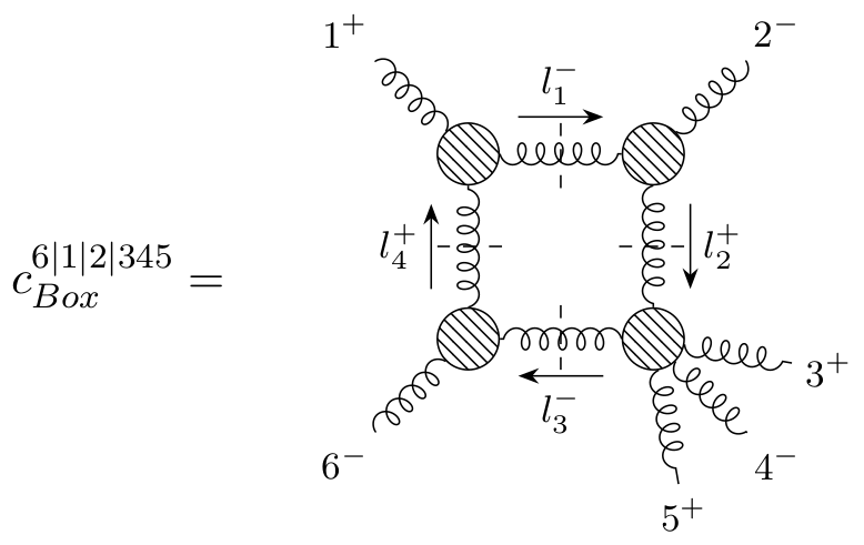
Multi-Loop Amplitudes from Trees

$\circ$ Generalized unitarity relates products of tree amplitudes to loop amplitudes
$$ \require{color} \displaystyle \prod_{\text{trees}} A^{\text{tree}}(\vec k, \vec\ell|_{\text{cut}}) = \sum_{\substack{\text{topologies}\, \Gamma, \\ i \in M_\Gamma \cup S_\Gamma}} \colorbox{yellow}{$c_{i,\Gamma}(\vec k)$} \left( \frac{m_{i,\Gamma}(\vec k, \vec\ell|_{\text{cut}})}{\displaystyle \prod_{\text{props}\,j} \rho_{j}(\vec k, \vec\ell|_{\text{cut}})} \right) $$ $$ \left. \begin{aligned} \underline{\text{Master integrals}}: \; & \int d^{D}\vec \ell \; \frac{m_{i\in M_\Gamma}}{\small \prod_j \rho_j} \neq 0 \\ \underline{\text{Surface terms}}: \; & \int d^{D}\vec \ell \; \frac{m_{i\in S_\Gamma}}{\small \prod_j \rho_j} = 0 \\ \end{aligned} \right\} \; \begin{aligned} & \text{Complex} \\ & \text{problem!} \end{aligned} $$


$\circ$ The diagram on the right shows as example a one-loop box coefficient.

$\circ$ In general, need to solve linear systems for the coefficients $c_{i,\Gamma}$.

Analytics from Numerics

Problem: direct analytic computation of the $c_{i,\Gamma}$ is not feasible.
$\circ\,$ Floating-point evaluations ($\mathbb{R}$ or $\mathbb{C}$) would be sufficient for phenomenology.
$\phantom{\circ}\,$ But they are so unstable, even this won't work.
$\circ\,$ Could try rational inputs ($\mathbb{Q}$), but integers grow way too large at intermediate stages.
$\circ\,$ Finite fields ($\mathbb{F}_p$) come to the rescue.
Peraro ('16) von Manteuffel, Schabinger ('14), 
$\phantom{\circ}\,$ These are integers modulo a prime number $p$ (no precision issue!):
$\phantom{\circ}\,$ $\mathbb{F}_p = \{0, 1, 2, \dots, p-1\} \quad \text{with operations} \quad \{+, -, \times, \div \}$
$\phantom{\circ}\,$ The prime $p$ needs to be large, to avoid accidental DivisionByZero .
$\circ\,$ But we can't do phenomenology with $\mathbb{F}_p$ !

Solution: sample $c_{i,\Gamma}$ in $\mathbb{F}_p$ $\;\Rightarrow\;$ reconstruct analytic expression for $c_{i,\Gamma}$

Finite Fields

$\circ\,$ Any rational number, other than multiples of $1/p$, has an equivalent in the finite field $\mathbb{F}_p$.

$\circ\,$ For example, let's work with $p=7$, i.e. with $\mathbb{F}_7 = \{0, 1, 2, 3, 4, 5, 6\}$:

$-1$ is the additive inverse of 1
$\Rightarrow \quad -1=6$ in $\mathbb{F}_7$, because $1+6 = 7 \, \% \, 7 = 0$
$\frac{1}{3}$ is the multiplicative inverse of 3
$\Rightarrow \quad \frac{1}{3}=5$ in $\mathbb{F}_7$, because $3 \times 5 = 15 \, \% \, 7= 1$
$\phantom{\circ}\,$ The Euclidean algorithm allows to compute inverses without checking every entry.
$\circ\,$ Numbers cannot grow out of control!
$\frac{14611884945785561885978841755360860231120837652831038320107}{1853742276676202006476394341472012983521981235200}=1251868773$ in $\mathbb{F}_{2147483647}$
$\phantom{\circ}\,$ $2147483647$ is $(2^{31}-1)$ which is the largest possible value $p$ working with 32-bits.

Analytic Reconstruction

Common-Denominator Ansatz

$\displaystyle c_{i,\Gamma}(\vec x) = \frac{\text{Num. poly}(\vec x)}{\text{Denom. poly}(\vec x)} = \frac{\text{Num. poly}(\vec x)}{\prod_j W_j(\vec x)}$
$\circ\,$ Interpolation in one variable (continued fraction)
Thiele (1909)

$c_{i,\Gamma}(t) = c_{i,\Gamma}(t_0) + \frac{t-t_0}{\frac{t_0 - t_1}{c_{i,\Gamma}(t_0)-c_{i,\Gamma}(t_1)}+\frac{t-t_2}{\dots + \frac{t-t_3}{\dots}}} = \frac{\text{Num. poly}(t)}{\text{Denom. poly}(t)}$
$\phantom{\circ}\,$ Match denominator factors of $c_{i,\Gamma}(t)$ to $W_j(t)$ $\Rightarrow$ obtain the denominator (this is the easy part).
$\circ\,$ The numerator is much more complicated, in general
For spinors: GDL, Maître (2019)
$\displaystyle \text{Num. poly}(\vec x) = \sum_{\vec \alpha} c_{\vec\alpha} \; x_1^{\alpha_1} \dots x_{m}^{\alpha_{m}}$
$\circ\,$ To solve the system must sample as many times as there are undertermined $c_{\vec\alpha}$'s.

Tools of the Trade

$\circ\,$ In practice, using spinors $m = n(n-1)$ and there are constraints on $\vec \alpha$
Gröbner bases $\rightarrow$ constrain $\vec\alpha$
Decker, Greuel, Pfister, Schönemann
Integer programming $\rightarrow$ enumerate sols. $\vec\alpha$

Perron and Furnon (Google optimization team)


$\circ\,$ Solving linear systems with CUDA in $\mathbb{C}$ or $\mathbb{F}_{p\leq 2^{31}-1}$ (currently private code)
System Size Timing
8192 8 s
16384 51 s
32768 6m 30s
with RTX 2080ti 11GB
the absolute maximum is 52440 unknowns

(thanks gpu-Merlin!)

Taming the Algebraic Complexity

Problem: the least-common-denominator form is overly complex.
Its numerator can easily exceed 1 million monomials (e.g. 5-point 1-mass processes).
$\circ\,$ For example, taking homogeneous expressions in 5 variables
$\displaystyle c_{i,\Gamma}(x_1, \dots, x_5) = \frac{\text{126 monomials of degree 5}}{x_1x_2x_3x_4x_5}$
$\phantom{\circ\,}$ but say we knew that $x_1x_2$ don't appear in the same denominator as the others, then
$\displaystyle c_{i,\Gamma}(x_1, \dots, x_5) = \frac{\text{15 monomials of degree 2}}{x_1x_2}+\frac{\text{35 monomials of degree 3}}{x_3x_4x_5}$
Goal: use partial-fraction decompositions,
but how to achieve this without an analytic expression?


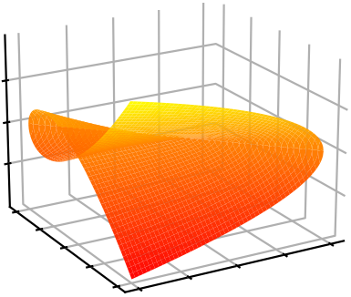
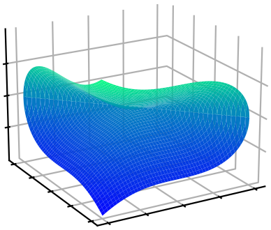
The Geometry of Phase Space


based on: GDL, Page (JHEP 12 (2022) 140)

Least Common Denominator Redux

$\circ\,$ Can't draw pictures in high (complex) dimensions, so let's consider the simplified case $\mathbb{R}[x, y, z]$.
$\circ\,$ Denominator factors $W_j$ correspond to singular surfaces .

${\color{orange}W_1 = (xy^2 + y^3 - z^2)}$
Say we have:
$W_1 = xy^2 + y^3 - z^2$
A function $c_i(x,y,z)$ may or may not have $W_1$ as a pole, depending on what happens on the orange surface
$\displaystyle \lim_{W_j \rightarrow \epsilon} c_i(x,y,z) \sim \frac{1}{\epsilon^{q_{ij}}} $


The LCD tells us about what happens on surfaces with one less dimension than the full space.

Multivariate Partial Fractions

$\circ\,$ To distinguish $\displaystyle \frac{1}{W_1W_2}$ from $\displaystyle \frac{1}{W_1} + \frac{1}{W_2}$, look at $W_1 \sim W_2 \rightarrow \epsilon \ll 1$. Geometrically:

${\color{orange}W_1 = (xy^2 + y^3 - z^2)}$

${\color{blue}W_2 = (x^3 + y^3 - z^2)}$

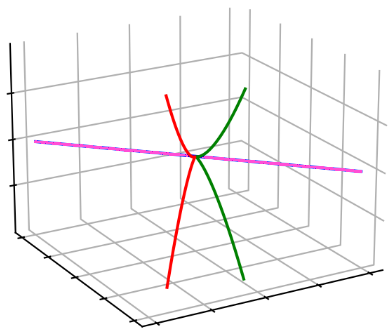
$V(W_1) \cap V(W_2)$
$\circ\,$ Primary decompositions of sets of polynomials ( ideals ), anogous to integers:
$60 = 5 \times 3 \times 2^2$
$({\color{orange}xy^2 + y^3 - z^2}, {\color{blue}x^3 + y^3 - z^2}) = \\ {\color{magenta}(z^2,x+y)} \cup {\color{green}(y^3-z^2,x)} \cup {\color{red}(2y^3-z^2,x-y)}$
Partial-fraction decompositions tell us about the relations between poles.
Upcoming Results
$\circ\,$ First two-loop computation in full color ($N_c$ dependence) for $q\bar q \rightarrow \gamma \gamma \gamma$
Kinematics # Poles ($W$) LCD Ansatz Partial-Fraction Ansatz Rational Functions
5-point massless 30 29k 4k $\sim$200 KB
$\circ\,$ Updated two-loop leading-color amplitudes for $pp \rightarrow Wjj$, now in spinor helicity
Kinematics # Poles ($W$) LCD Ansatz Partial-Fraction Ansatz Rational Functions
5-point 1-mass >200 >5M $\sim$40k $\sim$25 MB
$\phantom{\circ\,}$ First computed in Abreu, Febres Cordero, Ita, Klinkert, Page, Sotnikov (1.2 GB)

Try it yourself

pip install lips pyadic


Thanks for your attention!


Questions?

Backup Slides

Absolute Values
on the Rationals

$\boldsymbol p\,$-adic Numbers

$\circ\,$ We have again a problem in a finite field 1 is not smaller than 2. In fact:

$|x = 0|_{\mathbb{F}_p} = 0 \quad \text{and} \quad |x \neq 0|_{\mathbb{F}_p} = 1$
$\phantom{\circ}\,$ Can't easily take limits, without dividing by zero.

$\circ\,$ A $p$-adic number $x \in \mathbb{Q}_p$ is Laurent expansion in powers of the prime $p$
$x = a_{\nu_p} p^{\nu_p} + \dots + a_{-1}p^{-1} + a_{0} p^{0} + a_1 p^1 + \dots $
$\circ\,$ The $p$-adic absolute value is defined as (note the minus sign!)
$|x|_{\mathbb{Q}_p} = p^{-\nu_p} \quad \Rightarrow \quad |p|_{\mathbb{Q}_p} < |1|_{\mathbb{Q}_p} < |\frac{1}{p}|_{\mathbb{Q}_p}$
Retain integer arithmetics, while restoring the ability to take limits!

Python Packages

pyAdic

$\circ\,$ Pyadic provides flexible number types for finite fields and $p$-adic numbers in Python.
Related algorithms, such as rational reconstruction are also implemented.
 from pyadic import ModP
 from fractions import Fraction as Q
 ModP(Q(7, 13), 2147483647)
 <<< 1817101548 % 2147483647
 # Can also go back to rationals
 from pyadic.finite_field import rationalise
 rationalise(ModP(Q(7, 13), 2147483647))
 <<< Fraction(7, 13)

Lips

$\circ\,$ Lips is a phase-space generator and manipulator for 4-dimensional kinematics in any field, $\mathbb{C}, \mathbb{F}_p, \mathbb{Q}_p, \mathbb{Q}[i]$. It is particularly useful for spinor-helicity computations.
 from lips import Particles
 from lips.fields.field import Field
 # Random finite field phase space point, arbitrary multiplicity
 multiplicity = 5
 PSP = Particles(multiplicity, field=Field("finite field", 2 ** 31 - 1, 1), seed=0)
 # Evaluate an arbitrary complicated expression
 PSP("(8/3s23⟨24⟩[34])/(⟨15⟩⟨34⟩⟨45⟩⟨4|1+5|4])")
 <<< 683666045 % 2147483647
$\circ\,$ It can also be used to generate points in singular configuration.

Spinor Helicity

Representations of the Lorentz group

(Recall: $\mathfrak{so}(1, 3)_\mathbb{C} \sim \mathfrak{su}(2) \times \mathfrak{su}(2)$)
$(j_{-},j_{+})$ dim. name quantum field kinematic variable
(0,0) 1 scalar $h$ m
(0,1/2) 2 right-handed Weyl spinor $\chi_{R\,\alpha}$ $\lambda_\alpha$
(1/2,0) 2 left-handed Weyl spinor $\chi_L^{\,\dot\alpha}$ $\bar{\lambda}^{\dot\alpha}$
(1/2,1/2) 4 rank-two spinor/four vector $A^\mu/A^{\dot\alpha\alpha}$ $P^\mu/P^{\dot\alpha\alpha}$
(1/2,0)$\oplus$(0,1/2) 4 bispinor (Dirac spinor) $\Psi$ $u, v$

Spinor Covariants

Weyl spinors are sufficient for massless particles:

$\text{det}(P^{\dot\alpha\alpha})=m^2 \rightarrow 0 \quad \Longrightarrow \quad P^{\dot\alpha\alpha} = \bar\lambda^{\dot\alpha}\lambda^\alpha$.

In terms of 4-momentum components we have:

$$ \lambda\_\alpha=\frac{1}{\sqrt{p^0+p^3}}\begin{pmatrix}p^0+p^3 \\\ p^1+ip^2\end{pmatrix} \, , \;\;\; \lambda^\alpha=\epsilon^{\alpha\beta} \lambda_\beta =\frac{1}{\sqrt{p^0+p^3}}\begin{pmatrix}p^1+ip^2 \\\ -p^0+p^3\end{pmatrix} $$ $\bar\lambda\_{\dot\alpha}=\frac{1}{\sqrt{p^0+p^3}}\begin{pmatrix}p^0+p^3 \\\ p^1-ip^2\end{pmatrix} \, , \;\;\; \bar\lambda^{\dot\alpha}=\epsilon^{\dot\alpha\dot\beta}\bar\lambda_{\dot\beta}=\frac{1}{\sqrt{p^0+p^3}}\begin{pmatrix}p^1-ip^2 \\\ \-p^0+p^3\end{pmatrix}$
$$ \bar\lambda\_{\dot\alpha} = (\lambda\_\alpha)^* \quad if \quad p^i \in \mathbb{R}; \quad \quad \bar\lambda\_{\dot\alpha} \neq (\lambda\_\alpha)^* \quad if \quad p^i \in \mathbb{C} $$

Spinor Invariants

$$ ⟨ij⟩ = λ_iλ_j = (λ_i)^α(λ_j)_α \quad \quad \quad [ij] = \barλ_i\barλ_j = (\barλ_i)\_\dotα(\barλ_j)^\dotα $$ $$ s_{ij} = ⟨ij⟩[ji] $$ $$ ⟨i\;|\;(j+k)\;|\;l] = (λ_i)^α (\not P_j + \not P_k )\_{α\dotα} \barλ_l^\dotα $$ $$ ⟨i\;|\;(j+k)\;|\;(l+m)\;|\;n⟩ = (λ_i)^α (\not P_j + \not P_k )\_{α \dot α} (\bar{\not P_l} + \bar{\not P_m} )^{\dot α α} (λ_n)_α $$ $$ tr_5(ijkl) = tr(\gamma^5 \not P_i \not P_j \not P_k \not P_l) = [i\,|\,j\,|\,k\,|\,l\,|\,i⟩ - ⟨i\,|\,j\,|\,k\,|\,l\,|\,i] $$

Five-Parton Two-Loop
Finite Remainders


Example Simplifications

uubggg pmpmp Nf1 #3

is equal to $ -\frac{[32]^3 [41]^3}{2 [31]^3 [42]^3} $

ggggg mpmpp Nf1 # 9


is equal to
$-1\frac{[12]³[15][23]⟨25⟩³[35]³}{[13]⁴[25]⟨5|1+2|5]³}+\frac{97}{12}\frac{[12]⁴⟨25⟩[35]⁴}{[13]⁴[25]³⟨5|1+2|5]}$ $+\frac{13}{3}\frac{[12]⁴⟨15⟩[15][35]⁴}{[13]⁴[25]⁴⟨5|1+2|5]}+\frac{1}{4}\frac{[12]⁴⟨15⟩[15]⟨25⟩[35]⁴}{[13]⁴[25]³⟨5|1+2|5]²}$ $-\frac{3}{2}\frac{[12]²⟨25⟩²[25][35]²}{[13]²[25]⟨5|1+2|5]²}+\frac{7}{4}\frac{[12]³⟨25⟩²[35]³}{[13]³[25]⟨5|1+2|5]²}$ $-\frac{43}{3}\frac{[12]³⟨25⟩[35]³}{[13]³[25]²⟨5|1+2|5]}$ $-\frac{25}{3}\frac{[12]³⟨15⟩[15][35]³}{[13]³[25]³⟨5|1+2|5]}$ $-\frac{3}{2}\frac{[12]⟨25⟩[25][35]}{[13][25]⟨5|1+2|5]}$ $+4\frac{[12]²⟨25⟩[35]²}{[13]²[25]⟨5|1+2|5]}$ $-\frac{15}{2}\frac{[12]²[35]²}{[13]²[25]²}$ $+\frac{7}{2}\frac{[12][35]}{[13][25]}$ $-\frac{2}{3}$

Higgs + 4-Parton Amplitude
(@ finite top-mass)

Example of cut diagram

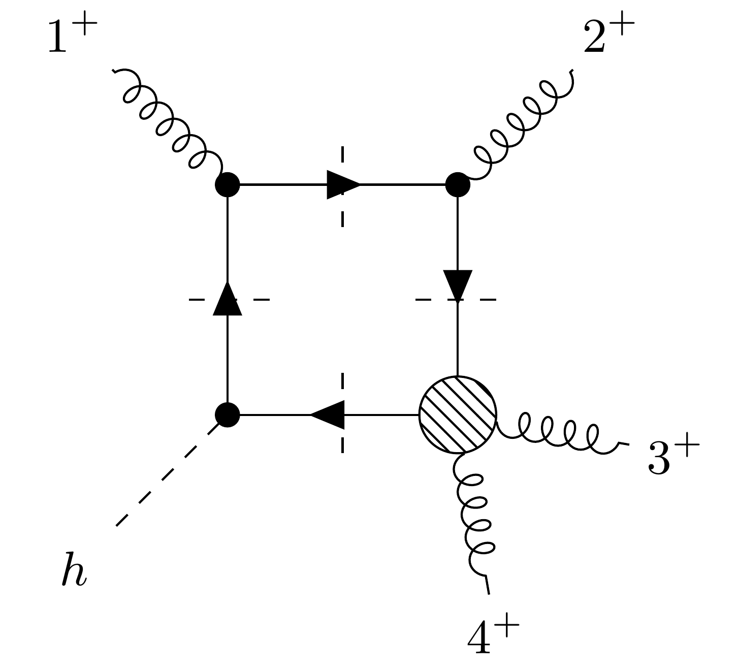
Only singularity involving $m_{top}$ (from pentagon contributions)

$16 |S_{1×2×3×4}| = −s_{12} , s_{23} , s_{34} , \langle 1 |2 + 3|4] , \langle 4|2 + 3|1] + m^2_{top} , tr_5(1234)^2$

We can generate point near this singularity in a similar fashion.

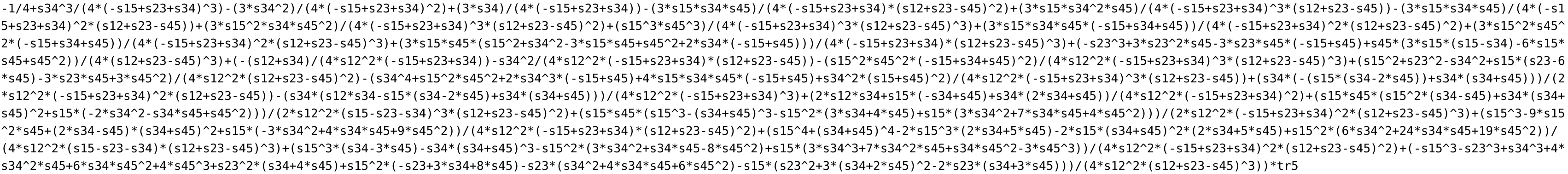
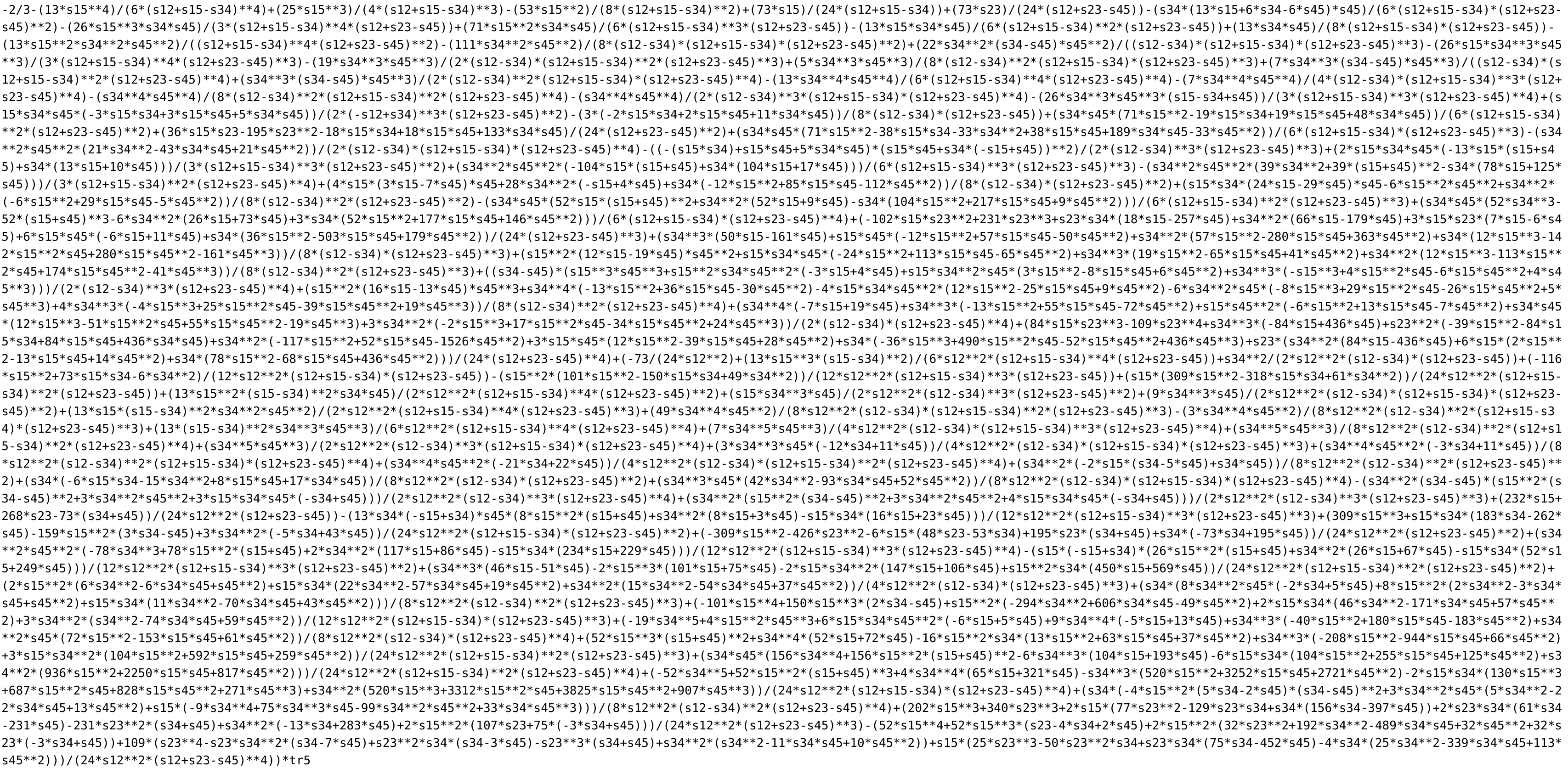
Structure of the coefficients

The massive external leg (the Higgs) is easily accomodated by considering it as a pair of massless particles (think decay products).
In the end all dependance on $P_{Higgs}$ is removed by using momentum conservation.

The coefficients are Taylor expasions in $m_{top}$:

$C^{(0)} + m^2_{top} C^{(2)}$.

with $C^{(0)}$ and $C^{(2)}$ resabling the six-gluon coefficients.