Scattering Amplitudes
$\circ$ Amplitude (integrands) can be written as
$$
\require{color}
\require{amsmath}
\displaystyle A(\lambda, \tilde\lambda, \ell) =
\sum_{\substack{\Gamma,\\ i \in M_\Gamma \cup S_\Gamma}} \, c_{\,\Gamma,i}(\lambda, \tilde\lambda, \epsilon) \, \frac{m_{\Gamma,i}(\lambda\tilde\lambda, \ell)}{\textstyle \prod_{j} \rho_{\,\Gamma,j}(\lambda\tilde\lambda, \ell)} \;\; \xrightarrow[]{\int d^D\ell} \;\; \sum_{\substack{\Gamma,\\ i \in M_\Gamma}} {\color{red}c_{\,\Gamma, i}}(\lambda, \tilde\lambda, \epsilon) \, {\color{orange}I_{\Gamma, i}}(\lambda\tilde\lambda, \epsilon)
$$
$\circ$ For a suitable choice of integrands, we get:
$$
\displaystyle
{\color{red}c_{\Gamma, i}}(\lambda, \tilde\lambda, \epsilon) = \frac{ \sum_{k=0}^{\text{finite}} \, {\color{red}c^{(k)}_{\,\Gamma, i}}(\lambda, \tilde\lambda) \, \epsilon^k}{\prod_j (\epsilon - a_{ij})} \;, \;\;\text{with} \quad a_{ij} \in \mathbb{Q}
$$
Some notation:
$\circ$ $\Gamma$: topologies $\quad\circ$ $M_\Gamma$: masters $\quad\circ$ $S_\Gamma$: surface terms
$\circ$ Spinors: $\lambda_i = |i\rangle, \tilde\lambda_i =[i|$
$\quad\circ$ 4-momenta: $\lambda\tilde\lambda=p\kern-3mm/$
$\quad\circ$ Loop $D$-momenta: $\ell $
Outline
Disclaimer: I will focus on the $c_{\,\Gamma, i}^{(k)}(\lambda, \tilde\lambda)$ $-$ call them $c_i(\lambda, \tilde\lambda)$ for short,
nevertheless some concepts can be extended to whole amplitudes.
We will discuss:
$1.$ Where are the $\color{red}\text{poles}$? What is their order?
$2.$ Relation between pole structure, and $\color{red}\text{analytic constraints}$ (e.g. partial fraction decomposition)
$3.$ Reconstructing $\color{red}\text{sets of functions}$: Why is it easier than reconstructing individual ones?
$4.$ Example process @ 2-loop: $\;\;pp \rightarrow \gamma\gamma\gamma\;\;$ and $\;\;pp \rightarrow Wjj\;\;$ (preliminary)
Key take away:
What is important is not the number of variables,
but the size of the parametrization (a.k.a. ansatz), and our ability to constrain it.
Polynomial Quotient Rings
$\circ$ Let us start from the polynomial ring of spinor components
$$\displaystyle \kern-50mm S_n = \mathbb{F}\left[|1⟩, [1|, \dots, |n⟩, [n|\right]$$
$\phantom{\circ}$ the field $\mathbb{F}$ can be any of $\mathbb{Q},\mathbb{R},\mathbb{C},\mathbb{F}_p,\mathbb{Q}_p,\dots$
$\circ$ Define the momentum-conservation ideal as
$$
\displaystyle J_{\Lambda_n} = \Big\langle \sum_i |i⟩[i| \Big\rangle_{S_n}
$$
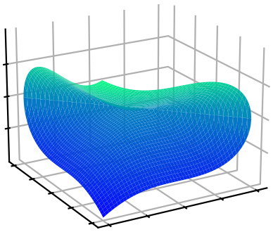
Artist's Impression of $V(J_{\Lambda_n})$
I can't draw in $4n$ dims!
$\phantom{\circ}$ physically, two polynomials $p$ and $q$ are equivalent if $p-q\in J_{\Lambda_n}$
$\circ$ This defines the needed polynomial quotient ring$\kern-4mm\phantom{x}^{\star}$: $\;R_n = S_n / J_{\Lambda_n} $
$c_i(\lambda, \tilde\lambda)$ at $n$-point belong to the Field of Fractions$\kern-4mm\phantom{x}^{\dagger}$ of $R_n$
$\kern-4mm\phantom{x}^\star R_4$ is "weird" (not a UFD), but it proves that polynomial rings are insufficient;
$\;\kern-4mm\phantom{x}^\dagger$ The field of fractions of $R_3$ does not exist.
Prime Ideals & Irreducible Varieties
$\circ$ Let us consider a very simple example
$\displaystyle \kern-50mm iA_{g^-g^-g^+g^+}^{\text{tree}} = \frac{\langle 12 \rangle^3}{\langle 23 \rangle \langle 34 \rangle \langle 41 \rangle} = \frac{[34]^3}{[12][23][41]} $
$\phantom{\circ}$ is, say, $\langle 23 \rangle$ a pole of this amplitude?
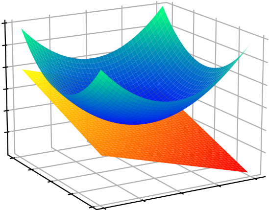
Artist's Impression of $V(\big\langle \langle 23 \rangle\big\rangle_{R_4})$
as the union of two irreducibles
$\circ$ The question is ill posed!
$\phantom{\circ} \langle 23 \rangle$ does not identify an irreducible variety in $R_4$.
$\phantom{\circ}$ Compute $\color{green}\text{primary decompositions}$, such as
$\displaystyle \big\langle \langle 23\rangle \big\rangle_{R_4} = {\color{orange} \big\langle \langle 23\rangle, [14] \big\rangle_{R_4}} \cap {\color{blue} \big\langle \langle 12\rangle, \langle 13 \rangle, \langle 14\rangle, \langle 23\rangle, \langle 24 \rangle, \langle 34 \rangle \big\rangle_{R_4}} $
$\phantom{\circ}$ On the first branch there is a simple pole, on the latter branch the amplitude is regular.
Poles & Zeros $\;\Leftrightarrow\;$ Irreducible Varieties $\;\Leftrightarrow\;$ Prime Ideals
Physics $\kern38mm$ Geometry $\kern38mm$ Algebra
Constraints from Poles
Bootstrapping trees (?)
$\circ$ The degree of divergence / vanishing on various surfaces imposes strong constraints, e.g.
$ A^{\text{tree}}_{q^+g^+g^+\bar q^-g^-g^-} = \frac{\mathcal{N(\text{m.d.} = 6\,,\; \text{p.w.} = [-1, 0, 0, 1, 0, 0])}}{\langle 12\rangle\langle 23\rangle\langle 34\rangle [45][56][61]s_{345}}$
$\circ$ Pretend this is un unknown integral coefficient, $\mathcal{N}$ has 143 free parameters.
$\circ$ List the various prime ideal, such as
$ \big\langle \langle 12\rangle, \langle 23\rangle, \langle 13\rangle \big\rangle, \; \big\langle |1\rangle \big\rangle, \; \big\langle \langle 12\rangle, |1+2|3]\big\rangle, \dots$
$\phantom{\circ}$ and impose that $\mathcal{N}$ vanishes to the correct order. We determine it up to an overall constant.
GDL, Page ('22)
$\circ$ Likewise, the ansatz for $A^{\text{tree}}_{g^+g^+g^+ g^-g^-g^-}$ shrinks $1326 \rightarrow 1$, etc..
Effectively, we can compute trees, just from their poles orders.
Note: compared to BCFW there is no information about residues.
Partial Fraction Decompositions
$\circ$ For true integral coefficients, we can't rely on the Ansatz to shrinks to an overall constant.
$\circ$ Partial fraction decompositions (PFDs) are a popular method to tame algebraic complexity.
$\circ$ In my opinion, a PFD algorithm needs
$1.$ to say if two poles $W_a$ and $W_b$ are separable into different fractions;
$2.$ ideally, to answer $(1.)$ without having access to an analytic expression.
$\circ$ Hilbert's nullstellensatz: if $\mathcal{N}$ vanishes on all branches of $\langle W_a, W_b \rangle$, then the PFD is possible$\kern-3mm\phantom{x}^\dagger$.
$\circ$ Generalizing to powers $>\kern-1mm 1$ can be done via symbolic powers and the Zariski-Nagata Theorem.
GDL, Page ('22)
$\circ$ Similarly, generalizing to non-radical ideals requires ring extensions.
Campbell, GDL, Ellis ('22)
Issue: evaluations on singular surfaces are expensive, but are not always needed!
Opportunity: we get more than partial fraction decompositions.
$\kern-4mm\phantom{x}^\dagger$ $\langle W_a, W_b\rangle$ needs to be radical.
Beyond Partial Fractions
$\circ$ $\color{red}\text{Case 0}$: the ideal does $\color{green}\text{not involve denominator factors}$.
E.g. a 6-point function $c_i$ has a pole at $⟨1|2+3|4]$ but not at $⟨4|2+3|1]$,
yet it is regular on the irreducible surface $V(\big\langle ⟨1|2+3|4], ⟨4|2+3|1] \big\rangle)$. Then
$\displaystyle c_i \sim \frac{⟨4|2+3|1]}{⟨1|2+3|4]} + \mathcal{O}(⟨1|2+3|4]^0) \; \text{ instead of } \; c_i \sim \frac{1}{⟨1|2+3|4]} + \mathcal{O}(⟨1|2+3|4]^0)$
$\circ$ $\color{red}\text{Case 1}$: the $\color{green}\text{degree of vanishing is non-uniform}$ across branches, for example:
$\displaystyle \frac{s_{14}-s_{23}}{⟨1|3+4|2]⟨3|1+2|4]}$
has a double pole on the first branch, and a simple pole on the second branch of
$\big\langle⟨1|3+4|2], ⟨3|1+2|4]\big\rangle_{R_6} = \big\langle ⟨13⟩, [24] \big\rangle_{R_6} \cap \big\langle ⟨1|3+4|2], ⟨3|1+2|4], (s_{14}-s_{23})\big\rangle_{R_6}$
$\circ$ $\color{red}\text{Case 2}$: ideal is $\color{green}\text{non-radical}$ (example on last slide)
$\displaystyle \small \kern0mm \sqrt{\big\langle {\color{black}⟨3|1+4|2]}, {\color{black}Δ_{23|14|56}} \big\rangle_{R_6}} = \big\langle {\color{black}⟨3|1+4|2]}, {\color{black}s_{124}-s_{134}} \big\rangle_{R_6} $
Choosing Independent Functions
$\circ$ The set $c_i$ can be very large, so pick a set of independent ones, and write:
$\displaystyle c_i = \tilde{c}_j M_{ji} \quad \text{with} \quad M_{ji} \in \mathbb{Q}$
$\phantom{\circ}$ with $\tilde{c}$ an independent subset of $c$.
$\phantom{\circ}\Longrightarrow$ $M_{ji}$ is, up to a permutation of columns, in row reduced echelon form.
$\circ$ We might as well use a set $\tilde{c}$ which is not a subset of $c$, at the trivial cost of changing $M_{ji}$.
$\circ$ Consider a PFD of one of the $\tilde{c}$'s:
$\displaystyle \tilde{c}_i(\lambda,\tilde\lambda) = \frac{\mathcal{N}_i(\lambda,\tilde\lambda)}{\prod_j W_j^{q_{ij}}(\lambda,\tilde\lambda)} = \sum_k \frac{\mathcal{N}_{ik}(\lambda,\tilde\lambda)}{\prod_j W_j^{q_{ijk}}(\lambda,\tilde\lambda)} = \sum_k \tilde{c}_{ik}(\lambda,\tilde\lambda)$
We $\color{red}\text{cannot have } \tilde{c}_i \in \text{span}(\tilde{c}_{j\neq i})$, but we $\color{green} \text{can have }\tilde{c}_{ik} \in \text{span}(\tilde{c}_{j\neq i})$, for some, but not all, $k$.
Least Least-Common-Denominator
$\circ$ In other words, the $\tilde{c}$ span a vector space, and we should $\color{green}\text{consider one modulo the others}$
$\displaystyle \tilde{c}_i = \sum_{j\neq i} q_j \tilde{c}_j + \tilde{c}'_{i}$
$\phantom{\circ}$ the basis function $\tilde{c}_i$ can be replaced by $\tilde{c}'_i$ without changing the vector space.
$\circ$ In particular, $\tilde{c}'_i$ needs not have all the poles of $\tilde{c}_i$, thus it can be much simpler.
$\phantom{\circ}$ In other words, $\color{red}\text{the LCD of }\tilde{c}'_i\text{ can be smaller than that of }\tilde{c}_i$.
$\circ$ Brute-force search works well when an analytic expressions is available.
$\circ$ In a future publication we will provide an algorithm based on finite field evaluations.
Reconstructing a set of $c_i$ is not as bad as reconstructing the most complex function in the set.
Three-photon production at two loops
$\circ\,$ The denominator factors $W_j$ are conjectured to be restricted to the letters of the symbol alphabet
Abreu, Dormans, Febres Cordero, Ita, Page ('18)
$\displaystyle \{W_j\} = \bigcup_{\sigma \; \in \; \text{Aut}(R_5)} \sigma \circ \big\{ \langle 12 \rangle, \langle 1|2+3|1] \big\} {\quad\color{green}\text{Identical to 1-loop!}}$
$\circ\,$ Advantage of spinor variables due to:
$1.$ little group covariant LCD (no spurious poles); $\;\;2.$ avoiding parity even/odd split;
$\Rightarrow\;$ in LCD form we would need $\color{green}29\,059$ evaluations instead of $\color{red}117\,810$ (with $s_{ij}$) for $\mathcal{R}^{(2)}_{2q3\gamma}$ .
$\circ\,$ To$\color{green}\text{ avoid evaluations on singular surfaces}$, use insights from physics (locality).
$\phantom{\circ}\,$ E.g. conjecture that no 5-point denominator has pairs of $\langle i |j + k | i]$, like at 1 loop.
$\circ$ Remove some overlap with other $\tilde{c}$'s, obtain the $\tilde{c}_i$ with higher degree LCD with $\color{green}4\,003$ points.
$\circ$ A posteriori, we find that for the $c_i$ with highest degree LCD the following would have sufficied
$\displaystyle \tilde{c}_i = \frac{⟨13⟩[14]^2⟨24⟩⟨34⟩[45]}{⟨45⟩⟨4|1+3|4]^3}-\frac{[14]⟨25⟩⟨34⟩^2[45]}{⟨45⟩^2⟨4|1+3|4]^2}-\frac{[14]⟨24⟩⟨34⟩⟨35⟩}{⟨45⟩^3⟨4|1+3|4]}$
W+2-jets: simplification strategy
$1.\,$ Script to split up the expressions, and compile them ($\sim 20$GB binaries) for evaluation over $\mathbb{F}_p$;
$2.\,$ Recombine the 3 projections $p_V \parallel p_1, p_V \parallel p_2, p_V \parallel p_3$ and reintroduce the little group factors
to build 6-point spinor-helicity amplitudes (subject to degree bounds on $|5\rangle,[5|,|6\rangle,[6|$);
$3.\,$ Perform (rough) PFDs based on expected structures and fit the Ansatze.
Comparison of $q\bar q \rightarrow \gamma \gamma \gamma$ (in full color) to $pp \rightarrow Wjj$ (at leading color):
| Kinematics |
# Poles ($W$) |
LCD Ansatz |
Partial-Fraction Ansatz |
Rational Functions |
| 5-point massless |
30 |
29k |
4k |
$\sim$300 KB |
| 5-point 1-mass |
>200 |
>5M |
$\sim$40k |
$\sim$25 MB |
$\displaystyle \kern-10mm \{W_j\} = \bigcup_{\sigma \; \in \; \text{Aut}(R_6)} \sigma \circ \big\{ \langle 12 \rangle, \langle 1|2+3|1], \langle 1|2+3|4], s_{123}, \Delta_{12|34|56}, ⟨3|2|5+6|4|3]-⟨2|1|5+6|4|2] \big\} $
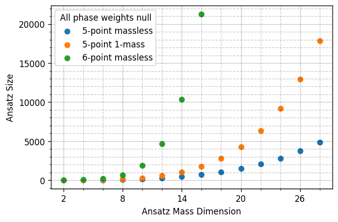
Analytic Structures of 2-loop 5-point 1-mass Amplitudes
$\circ$ The Ansatz size grows quickly with
multiplicity (m) and mass dimension (d):
$\displaystyle \small \left(\mkern -9mu \begin{pmatrix}\, m(m-3)/2 \, \\ \, d/2 \, \end{pmatrix} \mkern -9mu \right)$
is a lower bound.
GDL, Maître ('20)
$\circ\,$ Compact residues for the new 2-loop (spurious?) pole, $⟨k|j|p\mkern-7.5mu/_V|l|k]-⟨j|i|p\mkern-7.5mu/_V|l|j]$, e.g.:
$$r^{(5 \text{ of } 54)}_{\bar{u}^+g^+g^+d^-(V\rightarrow \ell^+ \ell^-)} = \frac{[12][23]⟨24⟩⟨46⟩^2⟨1|2+3|4]⟨2|1+3|4]}{⟨12⟩⟨23⟩⟨56⟩(⟨3|2|5+6|4|3]-⟨2|1|5+6|4|2])^2}$$
$\circ\,$ The three mass Grams, $\Delta_{12|34|p_V}, \Delta_{14|23|p_V}$, behave analogously to one-loop amplitudes, e.g.:
$$ r^{(73 \text{ of } 120)}_{\bar{u}^+g^-g^+d^-(V\rightarrow \ell^+ \ell^-)} = \frac{105}{128}\frac{⟨2|1+4|3]⟨4|2+3|1]⟨6|1+4|5]s_{14}s_{23}s_{56}{\color{green}(s_{124}-s_{134})}(s_{123}-s_{234})(s_{25}+s_{26}+s_{35}+s_{36})}{{\color{orange}⟨3|1+4|2]}{\color{red}Δ_{23|14|56}^4}} + \\
\Bigg[-6\frac{[12]^2⟨13⟩[25]⟨34⟩⟨36⟩⟨56⟩[56]{\color{green}(s_{124}-s_{134})}}{{\color{orange}⟨3|1+4|2]^5}}\Bigg] + \Bigg[ \; \Bigg]_{1234\rightarrow \overline{4321}}+ \mathcal{O}\left(\frac{1}{⟨3|1+4|2]^{4}Δ_{23|14|56}^{3}}\right)$$
Finite remainders & the
Rational / Transcendental split
$\circ$ In general, in $D= 4- 2 \epsilon$, with pure master integrals $I_{\Gamma, i}$ we have
$$ A^{\ell-loop}_n(\lambda, \tilde\lambda) = \sum_\Gamma \sum_{i \in M_\Gamma} \frac{\color{orange}{c_{\,\Gamma, i}}(\lambda, \tilde\lambda, \epsilon) \, \color{red}{I_{\Gamma, i}}(\lambda\tilde\lambda, \epsilon)}{\prod_j (\epsilon - a_{ij})}\;, \quad \text{with} \quad a_{ij} \in \mathbb{Q}$$
$\circ$ For NNLO applications, we are interested in the finite remainder
$$
\mathcal{A}^{(2)}_R = \underbrace{\mathcal{R}}_{\text{finite remainder}} + \underbrace{I^{(1)}\mathcal{A}^{(1)}_R \quad + \quad I^{(2)}\mathcal{A}^{(0)}_R}_{\text{divergent + convention-dependent finite part}} + \mathcal{O}(\epsilon)
$$
$$
\textstyle \mathcal{R}(\lambda, \tilde\lambda) = \sum_i \color{orange}{r_{i}(\lambda,\tilde\lambda)} \, \color{red}{h_i(\lambda\tilde\lambda)}
$$
Reconstruct $\color{orange}{r_{i}(\lambda,\tilde\lambda)}$ from $\mathbb{F}_p$ samples
Peraro ('16)
von Manteuffel, Schabinger ('14)
The Numerator Ansatz
$\circ\,$ The numerator Ansatz takes the form
GDL, Maître ('19)
$\displaystyle \text{Num. poly}(\lambda, \tilde\lambda) = \sum_{\vec \alpha, \vec \beta} c_{(\vec\alpha,\vec\beta)} \prod_{j=1}^n\prod_{i=1}^{j-1} \langle ij\rangle^{\alpha_{ij}} [ij]^{\beta_{ij}}$
$\phantom{\circ}$ subject to constraints on $\vec\alpha,\vec\beta$ due to: 1) mass dimension; 2) little group; 3) linear independence.
$\circ\,$ Construct the Ansatz via the algorithm from Section 2.2 of
GDL, Page ('22)
Linear independence = irreducibility by the Gröbner basis of a specific ideal.
$\circ\,$ Efficient implementation using open-source software only
$\circ\,$ All linear systems solved with CUDA over $\mathbb{F}_{p\leq 2^{31}-1}$ on a laptop ($t_{\text{solving}} \ll t_{\text{sampling}}$)
Polynomial Quotient Rings
vs.
Polynomial Rings
$\circ$ Can we get rid of equivalence relations (redundancies) by changing variables?
$\phantom{\circ}$ In other words, can we solve the redundancies and turn the quotient ring in a ring?
With four-point massless kinematics, you cannot. In $R_4$ we have
$ \langle 12\rangle [12] = \langle 34\rangle [34]$
this means that $R_4$ is not a unique factorization domain (UFD).
All polynomial rings are UFDs, so $R_4$ cannot be isomorphic to one.
The Field of Fractions of $R_3$ does not exists
$\circ$ $R_3$ is not an integral domain, i.e. there exists products of non-zero elements which are zero.
$\langle 12\rangle [23] = \langle 1|2|3] = -\langle 1| 1+3 |3] = 0 \;\text{but}\; \langle 12\rangle \neq 0 \;\text{and}\; [23] \neq 0$
Hence, one cannot define a field of fractions, as this would not be closed under multiplication.