Non-Planar Two-Loop Amplitudes
for Five-Parton Scattering

Giuseppe De Laurentis

University of Edinburgh

arXiv:2311.10086

(GDL, H. Ita, M. Klinkert, V. Sotnikov)

arXiv:2311.18752

(GDL, H. Ita, V. Sotnikov)

Loops & Legs 2024

Find these slides at gdelaurentis.github.io/slides/loopslegs_apr2024

Introduction

Overview

$\circ\,$ LHC physics program possible also thanks to advancements on many fronts of the theory

Subtraction
Pikelner, Pedron, Guadagni, Magnea, van Hameren, Vicini, $\dots$
Renomalization / $\gamma^5$-schemes
Gracey, Heinrich, Weißwange, Kühler, Stöckinger$\dots$
Feynman Integrals
Chaubey, Behring, Nega, Jones, Zoia, Banik, Page, Broadhurst, $\dots$

Three / Four / Five Loops
Bluemlein, Yang, Moch, Schönwald, Maier, $\dots$
$\sigma$'s at N$^{(2-3)}$LO
Sotnikov, Neumann, Chen, Mella, Savoini, $\dots$
Automation
Lange, Shtabovenko, Zoller$\dots$

Higgses ($2 \rightarrow 2$ w/ masses)
Zhang, Davies, Kerner, $\dots$
Top-quark(s), internal or external
Vitti, Coro, Wang, Magerya, $\dots$
Resummation
Novikov, Andersen, Li, $\dots$

And much more! Also, lines between various subfields often very blurry!

This talk: fixed order, 2 loops and 5 legs.

Precision Physics Requires NNLO Corrections

$\circ\,$ K-factors at NNLO can still be large, especially if new channels open up beyond tree, e.g. $\sigma^{\text{NNLO}}_{pp\rightarrow \gamma\gamma\gamma}$

Chawdhry, Czakon, Mitov, Poncelet ('19)

Kallweit, Sotnikov, Wiesemann ('20)

$\circ\,$ High-multiplicity two-loop amplitudes required also because:

$\qquad\star$ At high energy, some radiation is more likely than no radiation (resummation disrupts naive $\alpha_s$ counting)

$\qquad\star$ As real-virtual(-virtual) contributions to emerging N$^3$LO computations (or N$^2$LO if loop-induced)

$\qquad\star$ Some interesting kinematic regions are only accessible with extra radiation (e.g. $p_T$ distributions)

Status of Two-Loop Five-Point Amplitudes

Process	Analytical Amplitudes	Numerical Codes	Cross Sections
$pp \rightarrow \gamma\gamma\gamma$	[3$\kern-2.2mm\phantom{x}^\star$, 4$\kern-2.2mm\phantom{x}^\star$, 5]	[3$\kern-2.2mm\phantom{x}^\star$, 5]	[1$\kern-2.2mm\phantom{x}^\star$, 2$\kern-2.2mm\phantom{x}^\star$]
$pp \rightarrow \gamma\gamma j$	[6$\kern-2.2mm\phantom{x}^\dagger$, 7$\kern-2.2mm\phantom{x}^\dagger$, 9]	[6$\kern-2.2mm\phantom{x}^\dagger$]	[8$\kern-2.2mm\phantom{x}^\dagger$]
$pp \rightarrow \gamma jj$	[10]		[10]
$pp \rightarrow jjj$	[11$^\dagger$, 12, 13, 14]	[11$^\dagger$,14]	[15$\kern-2.2mm\phantom{x}^\dagger$, 16$\kern-2.2mm\phantom{x}^\dagger$]
$pp \rightarrow Wb\bar b$	[17$\kern-2.2mm\phantom{x}^\dagger$, 18$\kern-2.2mm\phantom{x}^{\dagger\ast}$, 19a$\kern-2.2mm\phantom{x}^\dagger$]		[19a$\kern-2.2mm\phantom{x}^\dagger$, 19b$\kern-2.2mm\phantom{x}^\dagger$]
$pp \rightarrow Hb\bar b$	[20$^{\dagger\ast}$]
$pp \rightarrow Wj\gamma$	[21$^\star$]
$pp \rightarrow Wjj$	[17$\kern-2.2mm\phantom{x}^\dagger$]
$pp \rightarrow ttH$			[22]

Legend: bold = full color; $\star$ = planar $\neq$ leading color; $\dagger$ = planar = leading color; $\ast$ = ($y_b \neq 0$, $m_b = 0; \text{or } W-\text{onshell}$)

[1] Chawdhry, Czakon, Mitov, Poncelet '19

[3] Abreu, Page, Pascual, Sotnikov '20

[5] Abreu, GDL, Ita, Klinkert, Page, Sotnikov '23

[7] Chawdhry, Czakon, Mitov, Poncelet '21

[9] Agarwal, Buccioni, von Manteuffel, Tancredi '21

[11] Abreu, Febres Cordero, Ita, Page, Sotnikov

[13] GDL, Ita, Klinkert, Sotnikov '23

[15] Czakon, Mitov, Poncelet '21'

[17] Abreu, Febres Cordero, Ita, Klinkert, Page, Sotnikov '21

[19a, 19b] Hartanto, Poncelet, Popescu, Zoia '22

[21] Badger, Hartanto, Kryś, Zoia '22

[2] Kallweit, Sotnikov, Wiesemann '20

[4] Chawdhry, Czakon, Mitov, Poncelet '20

[6] Agarwal, Buccioni, von Manteuffel, Tancredi '21

[8] Chawdhry, Czakon, Mitov, Poncelet '21

[10] Badger, Czakon, Hartanto, Moodie, Peraro, Poncelet, Zoia '23

[12] Agarwal, Buccioni, Devoto, Gambuti, von Manteuffel, Tancredi '23

[14] GDL, Ita, Sotnikov '23

[16] Chen, Gehrmann, Glover, Huss, Marcoli '22

[18] Badger, Hartanto, Zoia '21

[20] Badger, Hartanto, Kryś, Zoia '21

[22] Catani, Devoto, Grazzini, Kallweit, Mazzitelli, Savoini '22

Full $N_C $ motivation

3 is not that big! And certainly not close to $\infty$

Slc contributions to $pp\rightarrow jjj$ should be similar to blue curve.

Expect $\mathcal{O}(10\%)$ effect on duble-virtual hard function,
this is scheme dependant.

Effect on $\sigma^{\text{NNLO}}$ depends on size of $\mathcal{H}^{(2)}$.

Pheno. Goal

Stable and fast evaluations for cross sections

C++ Code available at

gitlab.com/five-point-amplitudes/FivePointAmplitudes-cpp

Analytics available at

zenodo.org/records/10142295 & zenodo.org/records/10231547

with Mathematica, Python and C++ scripts.

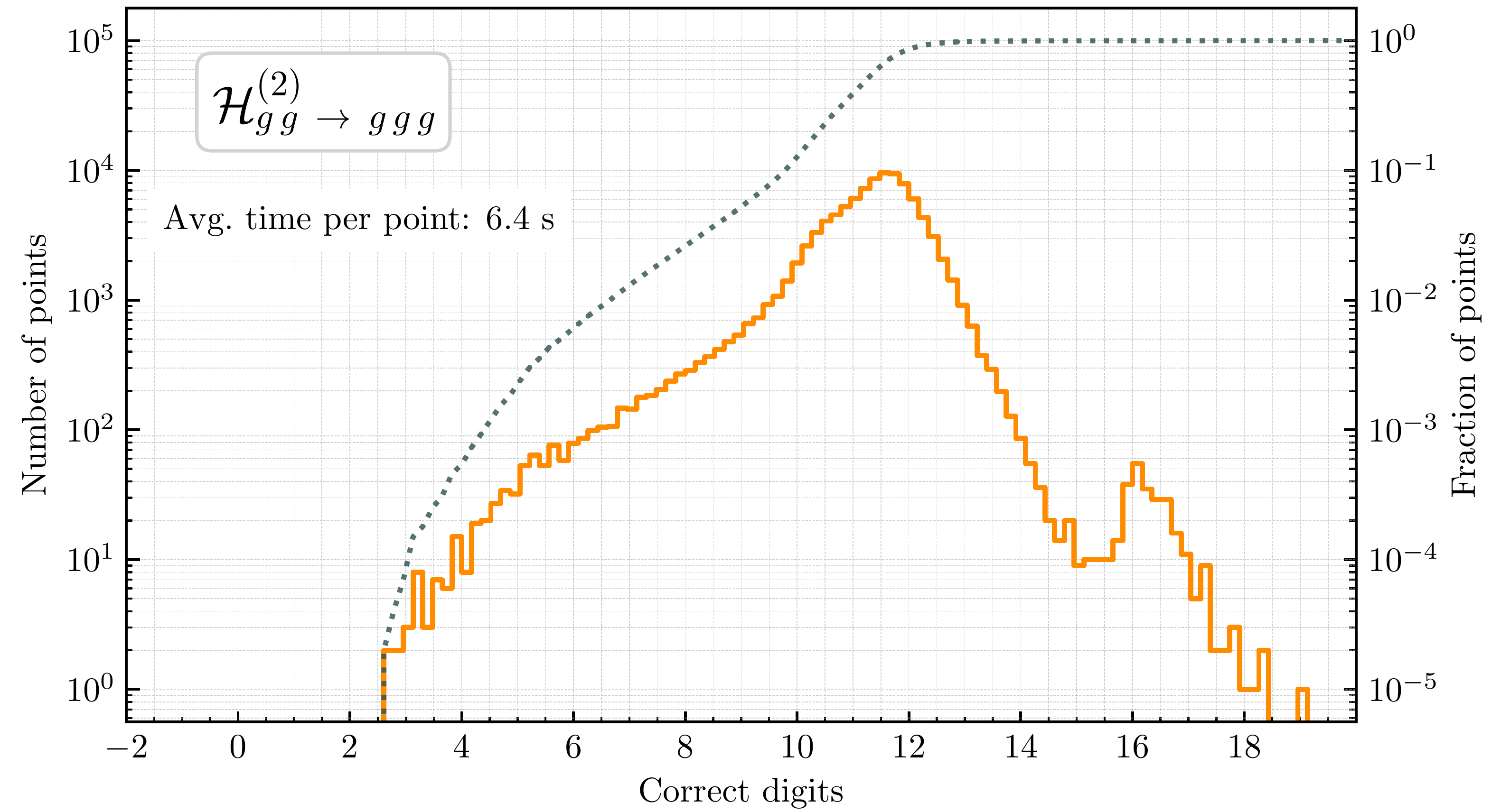
Numerical Computation

Color Algebra in the Trace Basis

\[ \require{color} \require{amsmath} \hspace{-5mm} \begin{align} \mathcal{A}_{\vec{a}}(1_g,2_g,3_g,4_g,5_g) & = \sum_{\sigma \in \mathcal{S}_5/\mathcal{Z}_5} \sigma\Big(\text{tr}(T^{a_1}T^{a_2}T^{a_3}T^{a_4}T^{a_5}) \; A_{1}(1,2,3,4,5)\Big) \; + \\[2mm] & \quad \sum_{\sigma\in \frac{\mathcal{S}_5}{\mathcal{Z}_2 \times \mathcal{Z}_3}} \sigma\Big(\text{tr}(T^{a_1}T^{a_2}) \text{tr}(T^{a_3}T^{a_4}T^{a_5}) \; A_{2}(1,2,3,4,5)\Big) + , \\[8mm] \mathcal{A}_{\vec{a}}(1_u,2_{\bar u},3_g,4_g,5_g) & = \sum_{\sigma \in \mathcal{S}_3(3,4,5)} \sigma\Big( (T^{a_3}T^{a_4}T^{a_5})^{\,\bar i_2}_{i_1} \; A_{3}(1,2,3,4,5)\Big) \; + \\[2mm] & \quad \sum_{\sigma \in \frac{\mathcal{S}_3(3,4,5)}{\mathcal{Z}_2(3,4)}} \sigma\Big(\text{tr}(T^{a_3}T^{a_4}) (T^{a_5})^{\,\bar i_2}_{i_1} \; A_{4}(1,2,3,4,5)\Big) \; + \\[2mm] & \quad \sum_{\sigma \in \frac{\mathcal{S}_3(3,4,5)}{\mathcal{Z}_{3}(3,4,5)}} \sigma\Big(\text{tr}(T^{a_3}T^{a_4}T^{a_5}) \delta^{\bar i_2}_{i_1} A_{5}(1,2,3,4,5)\Big) \; , \\[8mm] \mathcal{A}_{\vec{a}}(1_u,2_{\bar u},3_d,4_{\bar d},5_g) &= \sum_{\sigma \in \mathcal{Z}_2(\{1,2\},\{3,4\})} \sigma\Big( \delta^{\bar i_4}_{i_1} (T^{a_5})^{\,\bar i_2}_{i_3} \; A_{6}(1,2,3,4,5)\Big) \; + \\[2mm] & \quad \sum_{\sigma \in \mathcal{Z}_2(\{1,2\},\{3,4\})} \kern-2mm \sigma\Big( \delta^{\bar i_2}_{i_1} (T^{a_5})^{\,\bar i_4}_{i_3} \; A_{7}(1,2,3,4,5)\Big)\,,\kern-1mm \end{align} \]

Each $A_{i}$ has an expansion in powers of $\alpha_s$. We consider the $\alpha_s^2$ corrections.

Relations among Partials

$\circ$ $N_c^{n_c}$ & $N_f^{n_f}$ expansion, notation $A^{(L),(n_c, n_f)}_{\text{partial}}$, red = new, $0\rightarrow q\bar q Q\bar Q g$ example

\[ \begin{gather} A_6^{(2)} = N_c^2 A_6^{(2),(2,0)} + {\color{red} A_6^{(2),(0,0)}} + \frac{1}{N_c^2} {\color{red} A_6^{(2),(-2,0)}} + N_f N_c A_6^{(2),(1,1)} + \frac{N_f}{N_c} {\color{red} A_6^{(2),(-1,1)}} + N_f^2 A_6^{(2),(0,2)} \, , \\ A_7^{(2)} = N_c {\color{red} A_7^{(2),(1,0)}}+\frac{1}{N_c}{\color{red} A_7^{(2),(-1,0)}}+\frac{1}{N_c^3}{\color{red} A_7^{(2),(-3,0)}} + N_f{\color{red} A_7^{(2),(0,1)}} + \frac{N_f}{N_c^2} {\color{red} A_7^{(2),(-2,1)}} + \frac{N_f^2}{N_c}{\color{red} A_7^{(2),(-1,2)}} \, . \end{gather} \]

$\circ$ New identities among partials (plus two more for the $n_f = 1$ partials)

\[\\[2mm] \Big\{ \big[ 16 \, A^{(2),(2,0)}_6\, (1,2,3,4,5) + 4 \, A^{(2),(0,0)}_6\, (1,2,3,4,5) + A^{(2),(-2,0)}_6(1,2,3,4,5) \big] - \big[\dots \big]_{3 \leftrightarrow 4} \Big\} - \Big\{ \dots \Big\}_{1 \leftrightarrow 2} = 0 \, . \]

\[ \begin{gather} \big[ 32 \, A^{(2),(2,0)}_6\, (1,2,3,4,5) + 8 \, A^{(2),(0,0)}_6\, (1,2,3,4,5) + 2 A^{(2),(-2,0)}_6(1,2,3,4,5) \\ + 16 \, A^{(2),(1,0)}_7\, (1,2,3,4,5) \, + 4 A^{(2),(-1,0)}_7( 1,2,3,4,5) + A^{(2),(-3,0)}_7 (1,2,3,4,5) \big] - \big[ \dots \big]_{3 \leftrightarrow 4}= 0 \, . \end{gather} \]

These redundancies do not affect the complexity of the calculation (see discussion on vector spaces).

Partial Amplitudes & Finite Remainders

$\circ$ Amplitude (integrands) can be written as (for a suitable choice of master integrals)

$$ \displaystyle A(\lambda, \tilde\lambda, \ell) = \sum_{\substack{\Gamma,\\ i \in M_\Gamma \cup S_\Gamma}} \, c_{\,\Gamma,i}(\lambda, \tilde\lambda, \epsilon) \, \frac{m_{\Gamma,i}(\lambda\tilde\lambda, \ell)}{\textstyle \prod_{j} \rho_{\,\Gamma,j}(\lambda\tilde\lambda, \ell)} \;\; \xrightarrow[]{\int d^D\ell} \;\; \sum_{\substack{\Gamma,\\ i \in M_\Gamma}} \frac{ \sum_{k=0}^{\text{finite}} \, {\color{red}c^{(k)}_{\,\Gamma, i}}(\lambda, \tilde\lambda) \, \epsilon^k}{\prod_j (\epsilon - a_{ij})} \, {\color{orange}I_{\Gamma, i}}(\lambda\tilde\lambda, \epsilon) $$

$\circ$ $\Gamma$: topologies $\quad\circ$ $M_\Gamma$: master integrands $\quad\circ$ $S_\Gamma$: surface terms

$\circ$ All physical information is contained in the finite remainders, at two loops

Weinzierl ('11)

$$ \underbrace{\mathcal{R}^{(2)}}_{\text{finite remainder}} = \mathcal{A}^{(2)}_R \underbrace{- \quad I^{(1)}\mathcal{A}^{(1)}_R \quad - \quad I^{(2)}\mathcal{A}^{(0)}_R}_{\text{divergent + convention-dependent finite part}} + \mathcal{O}(\epsilon) $$

Catani ('98) Becher, Neubert ('09) Gardi, Magnea ('09)

$\phantom{\circ}$ $\mathcal{A}^{(1)}_R$ to order $\epsilon^2$ is still needed to build $\mathcal{R}^{(2)}$, but there is no real reason to reconstruct it.

$\circ$ Finite remainder as a weighted sum of pentagon functions Chicherin, Sotnikov ('20);

$$ \textstyle \mathcal{R}(\lambda, \tilde\lambda) = \sum_i \color{red}{r_{i}(\lambda,\tilde\lambda)} \, \color{orange}{h_i(\lambda\tilde\lambda)} $$

$\circ$ Goal: reconstruct $\color{red}{r_{i}(\lambda,\tilde\lambda)}$ from $\mathbb{F}_p$ samples

von Manteuffel, Schabinger ('14)
Peraro ('16)

Numerical Generalized Unitarity @ 2 Loops Ita (‘15) Abreu, Febres Cordero, Ita, Page, Zeng (‘17)

$\circ$ The integrand Ansatz is matched to products of trees on cuts

$$ \require{color} \displaystyle \sum_{\text{states}} \, \prod_{\text{trees}} A^{\text{tree}}(\lambda, \tilde\lambda, \ell)\big|_{\text{cut}_{\Gamma}} = \sum_{\substack{\Gamma' \ge \Gamma, \\ i \in M_\Gamma' \cup S_\Gamma'}} \kern-2mm c_{\,\Gamma',i}(\lambda, \tilde\lambda) \, \frac{m_{\Gamma',i}(\lambda\tilde\lambda, \ell)}{\displaystyle \prod_{j\in P_{\Gamma'} / P_{\Gamma}} \rho_{j}(\lambda\tilde\lambda, \ell)}\Bigg|_{\text{cut}_\Gamma} $$

C++ code

Abreu, Dormans,

Febres Cordero, Ita

Kraus, Page, Pascual,

Ruf, Sotnikov ('20)

$\star$ Numerical Berends-Giele recursion for LHS, solve for coeffs. in RHS.

$\star$ IBP reduction = decomposition on RHS, $\; m_{\Gamma,i} \in M_\Gamma \cup S_\Gamma $

$\circ$ The SLC cut-hierarchy is significantly larger than the LC one, e.g.

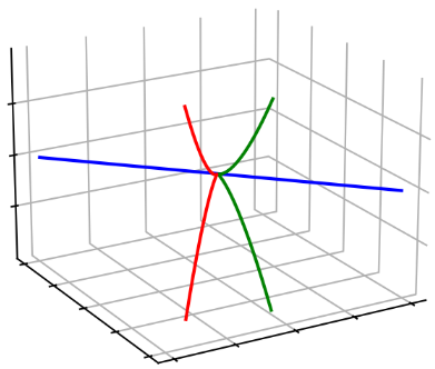
Analytic and Geometric Structure

based on:
GDL, Page (JHEP 12 (2022) 140)

Fieds of Fractions of Polynomial Quotient Rings

$\circ$ Starting from polynomials, we have

$\phantom{\circ}$ the covariant quotient ring of spinors

$$\displaystyle \kern10mm R_n = \mathbb{F}\big[|1⟩, [1|, \dots, |n⟩, [n|\big] \big/ \big\langle \sum_i |i⟩[i| \big\rangle$$

$\circ$ Lorentz invariants live in a sub-ring of $R_n$

$$\displaystyle \kern4mm R_n \supset \mathcal{R}_n = \mathbb{F}\big[⟨1|2⟩, \dots, [n-1|n]\big] \big/ (\mathcal{J}_n + \mathcal{K}_n + \bar{\mathcal{K}}_n)$$

$\phantom{\circ}$ where $\mathcal{J}_n$: momentum cons., $\;\stackrel{\tiny{(}\normalsize{-}\tiny{)}}{\mathcal{K}}_n$: shouten identities

Plot from LC $pp\rightarrow \gamma\gamma\gamma$ remainder in Born kinematics.

The slopes flatten out in soft/collinear configurations.

$r_i(\lambda, \tilde\lambda)$ at $n$-point belong to the field of fractions of $\mathcal{R}_{n>3}$

$\circ$ This allows to manifes:

$\kern8mm$ 1) that the singularities are $\approx \sqrt{s_{ij}}\kern10mm$ 2) the behaviour with $P^\mu \in \mathbb{C}$, i.e. away from $\langle ij \rangle = [ij]^{\ast}$

Least Common Denominator

(i.e. what happens at codimension one)

$\circ\,$ The rational coefficients take the form

$$ \displaystyle r_i(|i\rangle,[i|) = \frac{\mathcal{N}(|i\rangle,[i|)}{\prod_j \mathcal{D}_j^{q_{ij}}(|i\rangle,[i|)} $$

$\circ\,$ The $\mathcal{D}_j$ are related to the letters of the symbol alphabet

Abreu, Dormans, Febres Cordero, Ita, Page ('18)

$$ \displaystyle \{\mathcal{D}_{\{1,\dots,35\}}\} = \bigcup_{\sigma \; \in \; \text{Aut}(R_5)} \sigma \circ \big\{ \langle 12 \rangle, \langle 1|2+3|1] \big\} $$

$\kern0mm\color{green}\text{Identical to 1-loop!}$

The codimension one variety

$\langle x^3 + y^3 - z^2 \rangle$ in $\mathbb{R}[x,y,z]$

$\phantom{\circ}$ Non-trivial statement (not proven!): all irreducible polynomials generate prime ideals, @ 5-pt.

Poles & Zeros $\;\Leftrightarrow\;$ Irreducible Varieties $\;\Leftrightarrow\;$ Prime Ideals
Physics $\kern38mm$ Geometry $\kern38mm$ Algebra

Multivariate Partial Fraction Decompositions

(i.e. what happens at codimension greater than one)

$\langle xy^2 + y^3 - z^2 \rangle$

$\cap$

$\langle x^3 + y^3 - z^2 \rangle$

$=$

$\begin{gather}\langle 2y^3-z^2, x-y \rangle \cap \langle y^3-z^2, x \rangle \\ \cap \langle z^2, x+y \rangle\end{gather}$

$\circ$ When is a partial fraction decomposition possible? (an example)

$$\frac{\mathcal{N}}{(\prod_j \mathcal{D}_j^{q_j})\times\langle 4|1+3|4]\langle 5|1+4|5]} \stackrel{?}{=} \frac{\mathcal{N}_1}{(\prod_j \mathcal{D}_j^{q_j})\times\langle 4|1+3|4]} + \frac{\mathcal{N}_2}{(\prod_j \mathcal{D}_j^{q_j})\times\langle 5|1+4|5]}$$

$\circ$ Compute primary decompositions

$$ J = \big\langle \langle 4|1+3|4], \langle 5|1+4|5] \big\rangle \qquad K = \big\langle \langle14\rangle,\langle15\rangle,\langle45\rangle,[23] \big\rangle \quad L = \big\langle \langle ij\rangle \; \forall \; i,j\in\{1,\dots 5\} \big\rangle \\[2mm] M = \big\langle \langle 4|1+3|4], \langle 5|1+4|5], |1+4|5\rangle\langle14\rangle + |5|4\rangle\langle15\rangle, \langle\rangle \leftrightarrow [] \big\rangle $$

$$ J = K \cap \bar K \cap L \cap \bar L \cap M \quad \text{or} \quad V(J) = V(K) \cup V(\bar K) \cup V(L) \cup V(\bar L) \cap V(M) $$

If $\mathcal{N}$ vanishes on all branches than the equality holds by Hilbert's Nullstellensatz.

For a fleshed out example with open-source code see GDL (ACAT '22)

Analytic Reconstruction

see also tomorrow’s talks by Chawdhry and Liu

also based on:
GDL, Ita, Page, Sotnikov (to appear)

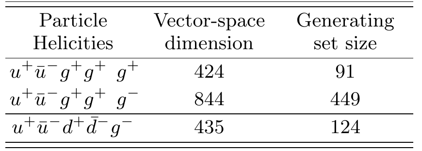
Vector Spaces of Rational Functions

$\circ\,$ Sort the $r_i$ by mass dimension of $\mathcal{N}$ ($\approx$ Ansatz size), pick simplest subset forming a basis $r_{i \in \mathcal{B}}$

$$ R = r_j h_j = r_{i\in \mathcal{B}} M_{ij} h_j \, , \qquad M_{ij} \in \mathbb{Q} $$

$\circ\,$ Change basis:

$$ \kern-20mm \tilde{r}_i = O_{ii'}r_{i'\in\mathcal{B}} \; \longrightarrow \; R = \tilde{r}_{i} \, O_{ii'}^{-1}M_{i'j} \, h_j = \tilde{r}_{i} \tilde{M}_{ij} h_j $$

$\circ\,$ Key insight to build a good $O_{ii'}:$

$$ \text{dim(span}(\lim_{\mathcal{D_j} \rightarrow 0 }r_{i})) \leq \text{dim(span}(r_{i})) $$

$\phantom{\circ}\,$ i.e., the pole residues are correlated, build linear combinations that de-correlate them

De-correlating the Residues

$\circ\,$ Build Laurent expansions around $t_{\mathcal{D}_k}$

$$ r_{i \in \mathcal{B}} = \sum_{m = 1}^{q_k = \text{max}_i(q_{ik})} \frac{e^k_{im}}{(t-t_{\mathcal{D}_k})^m} + \mathcal{O}((t-t_{\mathcal{D}_k})^0) $$

$\phantom{\circ}\,$ strictly formal over $\mathbb{F}_p$, but convergent over $\mathbb{Q}_p$ for $(t-t_{\mathcal{D}_k}) \propto p$

$\circ\,$ By Gaussian elimination, partition the space:

$$ \text{span}(r_{i \in \mathcal{B}}) = \underbrace{\text{column}(\text{Res}(r_{i \in \mathcal{B}}, \mathcal{D}_k^m))}_{\text{functions with the singularity}} \;\;\; \oplus \, \underbrace{\text{null}(\text{Res}(r_{i \in \mathcal{B}}, \mathcal{D}_k^m))}_{\text{functions without the singularity}} $$

$\circ\,$ Search for linear combinations that remove as many singularities as possible

$$ \kern25mm \displaystyle O_{i'i} = \bigcap_{k, m} \, \text{nulls}(\text{Res}(r_{i \in \mathcal{B}}, \mathcal{D}_k^m)) $$

Spinor-Helicity Results

$\circ$ The gluon MHV rational functions fit in 3 pages of the appendix

$$ \tilde{r}^{\text{MHV}}_{\text{first 5 of 115}} = \left\{ \frac{⟨45⟩^2}{⟨12⟩⟨13⟩⟨23⟩}, \frac{⟨45⟩^3}{⟨12⟩^2⟨34⟩⟨35⟩}, \frac{⟨45⟩^3}{⟨12⟩⟨15⟩⟨23⟩⟨34⟩}, \frac{[14][12][35]}{⟨23⟩[45]^3}, \frac{⟨45⟩^2⟨24⟩}{⟨12⟩^2⟨23⟩⟨34⟩}, \dots \right\} \text{+ symmetries}$$

$\circ$ All rational functions fitted in a single finite field. The matrices still required a few values of $p$.

$\circ$ The size of the results is dominated by the rational matrices (explicitly given for all crossings).

$\circ$ The simplification of the basis change is independent of that from PFDs.

$\circ$ Can now study propertities of the amplitude
$\phantom{\circ}$ e.g. no function has a $\text{tr}_5$ singularity, nor a pair of $\langle i | j + k | i]$ in the same denominator.

Quarks from Gluons

$\circ$ Checking whether a rational function belongs to a given vector space

$$ r_{\text{guess}} \stackrel{?}{\in} \text{span}_{FF(R_5), \mathbb{Q}}(r_{i}) $$

$\phantom{\circ}$ is much simpler problem than performing a rational reconstruction!
$\phantom{\circ}$ It only requires as many evaluations as the dimension of the vector space.

$\circ$ The vector space has uniform mass dimension and phase weights, which depend on helicities

$$ |i⟩ \rightarrow t^{1/2}|i⟩, \; |i] \rightarrow t^{1/2}|i] \quad \forall \; i \quad \text{and} \quad |i⟩ \rightarrow t|i⟩, \; |i] \rightarrow \frac{1}{t}|i] $$

$\circ$ Rescale gluon amplitudes in a way reminiscent of supersymmetry Ward identities

Elvang, Huang '13 $\;$

see e.g. $\;$

$$ \tilde{r}^{-}_{73}(q^+,q^-,g^+,g^+,g^-) = \frac{[14]⟨25⟩⟨45⟩}{⟨24⟩[24]⟨34⟩^2} = \frac{⟨14⟩}{⟨24⟩} \underbrace{\frac{[14]⟨25⟩⟨45⟩}{⟨14⟩[24]⟨34⟩^2}}_{r^{--}_{18}(g^+,g^-,g^+,g^+,g^-)} $$

$\circ$ We obtain most (50% of 2q3g and 90% of 4q1g) quarks functions this way.

Outlook

Complexity of 2-loop 5-point 1-mass Amplitudes

$\circ\,$ The number of letters in the spinor alphabet goes from 35 to more then 220:

$$ \displaystyle \kern5mm \{W_j\} = \bigcup_{\sigma \; \in \; \text{Aut}(R_6)} \sigma \circ \big\{ \langle 12 \rangle, \langle 1|2+3|1], \langle 1|2+3|4], s_{123}, \Delta_{12|34|56}, ⟨3|2|5+6|4|3]-⟨2|1|5+6|4|2] \big\} $$

$\phantom{\circ}\,$ from the point of view of the coefficients, this is closer to a massless 6-pt. computation than a 5-pt. one.

$\circ$ The LCD Ansatz size grows quickly with
multiplicity (m) and mass dimension (d):

GDL, Maître ('20)
$\displaystyle \kern20mm \text{Ansatz size} \geq \small \left(\mkern -9mu \begin{pmatrix}\, m(m-3)/2 \, \\ \, d/2 \, \end{pmatrix} \mkern -9mu \right)$

$\circ\,$ We can still achieve compact results, e.g. for the new (spurious?) 2-loop pole, $⟨k|j|p\mkern-7.5mu/_V|l|k]-⟨j|i|p\mkern-7.5mu/_V|l|j]$ $$r^{(5 \text{ of } 54)}_{\bar{u}^+g^+g^+d^-(V\rightarrow \ell^+ \ell^-)} = \frac{[12][23]⟨24⟩⟨46⟩^2⟨1|2+3|4]⟨2|1+3|4]}{⟨12⟩⟨23⟩⟨56⟩(⟨3|2|5+6|4|3]-⟨2|1|5+6|4|2])^2}$$

Iterated Reconstruction by Sequentially Removing Poles

$\circ\,$ In general results are much more complicated, but we can retain control surface-by-surface

Campbell, GDL, Ellis, ('22)

and $\;$

GDL, Page ('22) $\;$

Backup Slides

Constraints from Poles
Bootstrapping trees (?)

$\circ$ The degree of divergence / vanishing on various surfaces imposes strong constraints, e.g.

$ A^{\text{tree}}_{q^+g^+g^+\bar q^-g^-g^-} = \frac{\mathcal{N(\text{m.d.} = 6\,,\; \text{p.w.} = [-1, 0, 0, 1, 0, 0])}}{\langle 12\rangle\langle 23\rangle\langle 34\rangle [45][56][61]s_{345}}$

$\circ$ Pretend this is un unknown integral coefficient, $\mathcal{N}$ has 143 free parameters.

$\circ$ List the various prime ideal, such as

$ \big\langle \langle 12\rangle, \langle 23\rangle, \langle 13\rangle \big\rangle, \; \big\langle |1\rangle \big\rangle, \; \big\langle \langle 12\rangle, |1+2|3]\big\rangle, \dots$

$\phantom{\circ}$ and impose that $\mathcal{N}$ vanishes to the correct order. We determine it up to an overall constant.

GDL, Page ('22)

$\circ$ Likewise, the ansatz for $A^{\text{tree}}_{g^+g^+g^+ g^-g^-g^-}$ shrinks $1326 \rightarrow 1$, etc..

Effectively, we can compute trees, just from their poles orders.
Note: compared to BCFW there is no information about residues.

Partial Fraction Decompositions

$\circ$ For integral coefficients, we can't rely on the Ansatz to shrinks to an overall constant.

$\circ$ Partial fraction decompositions (PFDs) are a popular method to tame algebraic complexity.

$\circ$ In my opinion, a PFD algorithm needs

$1.$ to say if two poles $W_a$ and $W_b$ are separable into different fractions;
$2.$ ideally, to answer $(1.)$ without having access to an analytic expression.

$\circ$ Hilbert's nullstellensatz: if $\mathcal{N}$ vanishes on all branches of $\langle W_a, W_b \rangle$, then the PFD is possible$\kern-3mm\phantom{x}^\dagger$.

$\circ$ Generalizing to powers $>\kern-1mm 1$ can be done via symbolic powers and the Zariski-Nagata Theorem.

GDL, Page ('22)

$\circ$ Similarly, generalizing to non-radical ideals requires ring extensions.

Campbell, GDL, Ellis ('22)

Issue: evaluations on singular surfaces are expensive, but are not always needed!

Opportunity: we get more than partial fraction decompositions.

$\kern-4mm\phantom{x}^\dagger$ $\langle W_a, W_b\rangle$ needs to be radical.

Beyond Partial Fractions

$\circ$ $\color{red}\text{Case 0}$: the ideal does $\color{green}\text{not involve denominator factors}$.

E.g. a 6-point function $c_i$ has a pole at $⟨1|2+3|4]$ but not at $⟨4|2+3|1]$,

yet it is regular on the irreducible surface $V(\big\langle ⟨1|2+3|4], ⟨4|2+3|1] \big\rangle)$. Then

$\displaystyle c_i \sim \frac{⟨4|2+3|1]}{⟨1|2+3|4]} + \mathcal{O}(⟨1|2+3|4]^0) \; \text{ instead of } \; c_i \sim \frac{1}{⟨1|2+3|4]} + \mathcal{O}(⟨1|2+3|4]^0)$

$\circ$ $\color{red}\text{Case 1}$: the $\color{green}\text{degree of vanishing is non-uniform}$ across branches, for example:

$\displaystyle \frac{s_{14}-s_{23}}{⟨1|3+4|2]⟨3|1+2|4]}$

has a double pole on the first branch, and a simple pole on the second branch of

$\big\langle⟨1|3+4|2], ⟨3|1+2|4]\big\rangle_{R_6} = \big\langle ⟨13⟩, [24] \big\rangle_{R_6} \cap \big\langle ⟨1|3+4|2], ⟨3|1+2|4], (s_{14}-s_{23})\big\rangle_{R_6}$

$\circ$ $\color{red}\text{Case 2}$: ideal is $\color{green}\text{non-radical}$ (example on last slide)

$\displaystyle \small \kern0mm \sqrt{\big\langle {\color{black}⟨3|1+4|2]}, {\color{black}Δ_{23|14|56}} \big\rangle_{R_6}} = \big\langle {\color{black}⟨3|1+4|2]}, {\color{black}s_{124}-s_{134}} \big\rangle_{R_6} $

The Numerator Ansatz

$\circ\,$ The numerator Ansatz takes the form

GDL, Maître ('19)

$\displaystyle \text{Num. poly}(\lambda, \tilde\lambda) = \sum_{\vec \alpha, \vec \beta} c_{(\vec\alpha,\vec\beta)} \prod_{j=1}^n\prod_{i=1}^{j-1} \langle ij\rangle^{\alpha_{ij}} [ij]^{\beta_{ij}}$

$\phantom{\circ}$ subject to constraints on $\vec\alpha,\vec\beta$ due to: 1) mass dimension; 2) little group; 3) linear independence.

$\circ\,$ Construct the Ansatz via the algorithm from Section 2.2 of GDL, Page ('22)

Linear independence = irreducibility by the Gröbner basis of a specific ideal.

$\circ\,$ Efficient implementation using open-source software only

Gröbner bases $\rightarrow$ constrain $\vec\alpha,\vec\beta$
Decker, Greuel, Pfister, Schönemann

Integer programming $\rightarrow$ enumerate sols. $\vec\alpha,\vec\beta$
Perron and Furnon (Google optimization team)

$\circ\,$ Linear systems solved w/ CUDA over $\mathbb{F}_{2^{31}-1}$ ($t_{\text{solving}} \ll t_{\text{sampling}}$) w/ linac (coming soon-ish)