Cross Sections
Motivations
$\circ$ tri-jet @ $\text{NNLO}$;
$\circ$ di-jet @ $\text{N}^3\text{LO}$;
$\circ$ $\alpha_s$ extraction;
$\circ$ collinear factorization breaking (?);
$\circ$ multi-Regge kinematic limit;
$\circ \; \dots$
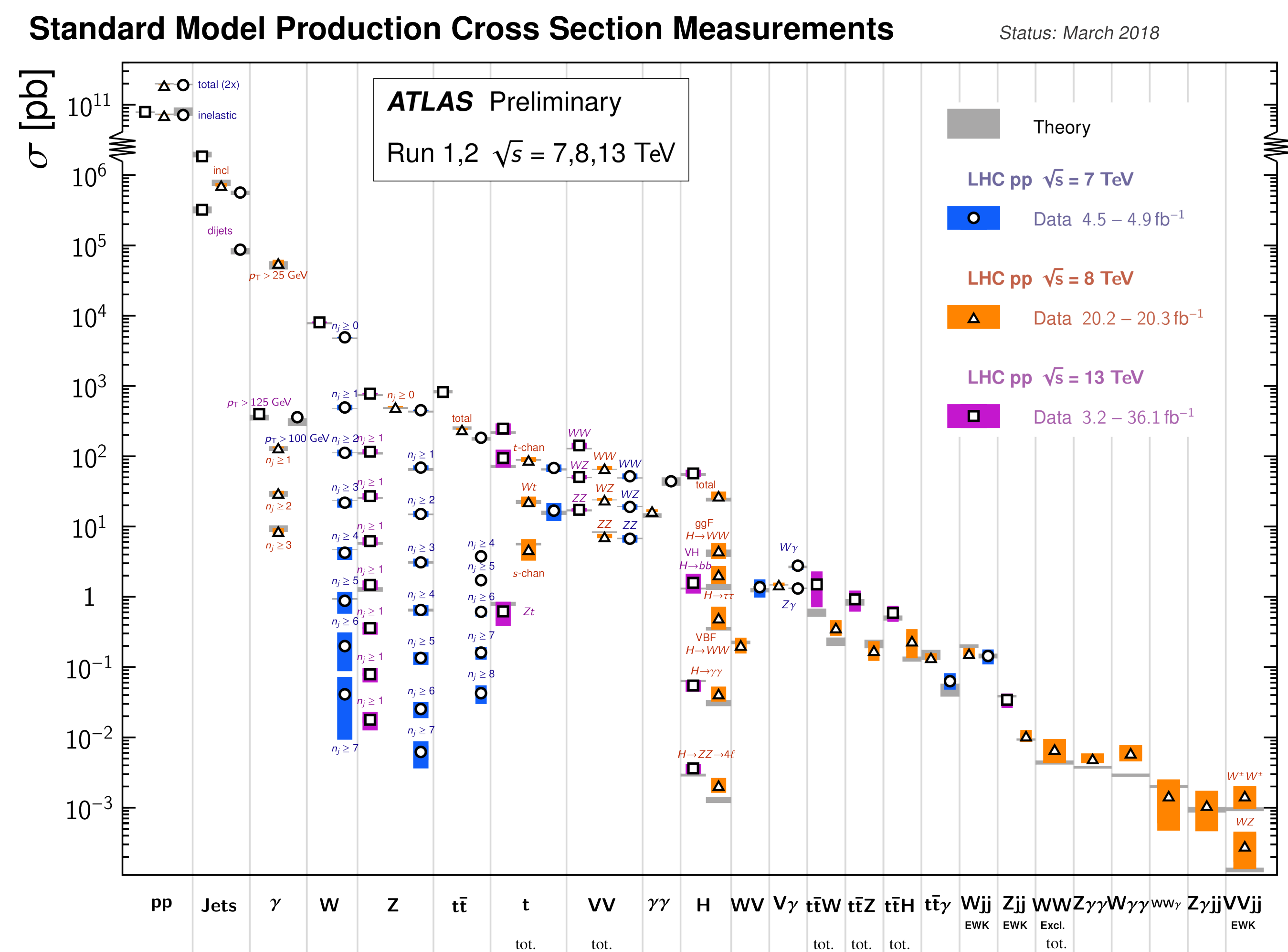
ATLAS Cross-Sections Summary
$$
σ_{2 \rightarrow n - 2} = \sum_{a,b} \int dx_a dx_b f_{a/h_1}(x_a, \mu_F) \, f_{b/h_2}(x_b, \mu_F) \;\hat{\sigma}_{ab\rightarrow n-2}(x_a, x_b, \mu_F, \mu_R)
$$
$$
\hat{σ}_{n}=\frac{1}{2\hat{s}}\int d\Pi_{n-2}\;(2π)^4δ^4\big(\sum_{i=1}^n p_i\big)\;|\overline{\mathcal{A}(p_i,h_i,a_i,μ_F, μ_R)}|^2
$$
Color Decompositions: ‘‘Trace’’ Basis
\[
\require{color}
\require{amsmath}
\hspace{-5mm}
\begin{align}
\mathcal{A}_{\vec{a}}(1_g,2_g,3_g,4_g,5_g) & = \sum_{\sigma \in \mathcal{S}_5/\mathcal{Z}_5} \sigma\Big(\text{tr}(T^{a_1}T^{a_2}T^{a_3}T^{a_4}T^{a_5}) \; A_{1}(1,2,3,4,5)\Big) \; + \\[2mm]
& \quad \sum_{\sigma\in \frac{\mathcal{S}_5}{\mathcal{Z}_2 \times \mathcal{Z}_3}} \sigma\Big(\text{tr}(T^{a_1}T^{a_2}) \text{tr}(T^{a_3}T^{a_4}T^{a_5}) \; A_{2}(1,2,3,4,5)\Big) + , \\[8mm]
\mathcal{A}_{\vec{a}}(1_u,2_{\bar u},3_g,4_g,5_g) & =
\sum_{\sigma \in \mathcal{S}_3(3,4,5)} \sigma\Big(
(T^{a_3}T^{a_4}T^{a_5})^{\,\bar i_2}_{i_1} \;
A_{3}(1,2,3,4,5)\Big) \; + \\[2mm]
& \quad \sum_{\sigma \in \frac{\mathcal{S}_3(3,4,5)}{\mathcal{Z}_2(3,4)}}
\sigma\Big(\text{tr}(T^{a_3}T^{a_4}) (T^{a_5})^{\,\bar i_2}_{i_1}
\; A_{4}(1,2,3,4,5)\Big) \; + \\[2mm]
& \quad \sum_{\sigma \in \frac{\mathcal{S}_3(3,4,5)}{\mathcal{Z}_{3}(3,4,5)}}
\sigma\Big(\text{tr}(T^{a_3}T^{a_4}T^{a_5}) \delta^{\bar i_2}_{i_1}
A_{5}(1,2,3,4,5)\Big) \; , \\[8mm]
\mathcal{A}_{\vec{a}}(1_u,2_{\bar u},3_d,4_{\bar d},5_g) &=
\sum_{\sigma \in \mathcal{Z}_2(\{1,2\},\{3,4\})} \sigma\Big(
\delta^{\bar i_4}_{i_1} (T^{a_5})^{\,\bar i_2}_{i_3}
\; A_{6}(1,2,3,4,5)\Big) \; + \\[2mm]
& \quad \sum_{\sigma \in \mathcal{Z}_2(\{1,2\},\{3,4\})} \kern-2mm \sigma\Big(
\delta^{\bar i_2}_{i_1} (T^{a_5})^{\,\bar i_4}_{i_3}
\; A_{7}(1,2,3,4,5)\Big)\,,\kern-1mm
\end{align}
\]
Each $A_{i}$ has an expansion in powers of $\alpha_s$. We consider the $\alpha_s^2$ corrections.
Color Decompositions: $N_c^{n_c}N_f^{n_f}$ Expansion
Notation = $A_{\scriptscriptstyle \#}^{(L),(n_c, n_f)}$; $\quad$ Red = New; $\quad$ leading color: $n_c + n_f = L$
\[
\begin{gather}
\sim\sim\sim\sim 5g \sim\sim\sim\sim\sim
\end{gather}
\]
\[
\begin{gather}
A_1^{(0)} = A^{(0),(0,0)} \, , \quad A_2^{(0)} = 0 \, , \qquad
A_1^{(1)} = N_c A^{(1),(1,0)} + N_f A^{(1),(0,1)} \, , \quad A_2^{(1)} = A^{(1),(0,0)} \,, \\[3mm]
A_1^{(2)} = N_c^2~A_1^{(2),(2,0)} ~+~ {\color{red} {A_1^{(2),(0,0)}}} + N_c N_fA_1^{(2),(1,1)} + N_c^{-1}N_f ~ {\color{red} {A_1^{(2),(-1,1)}}} + N_f^2 A_1^{(2),(0,2)} \,, \\[3mm]
A_2^{(2)} = N_c {\color{red} {A_2^{(2),(1,0)}}} +~ N_f {\color{red} {A_2^{(2),(0,1)}}} ~+~ N_c^{-1}N_f^2 {\color{red} {A_2^{(2),(-1,2)}} }\,.
\end{gather}
\]
\[
\begin{gather}
\sim\sim\sim\sim 2q3g \sim\sim\sim\sim\sim
\end{gather}
\]
\[
\hspace{-10mm}
\begin{gather}
A_3^{(0)} = A_3^{(0),(0,0)} \,, \quad A_4^{(0)} = 0\,, \quad A_5^{(0)} = 0\,, \\[4mm]
A_3^{(1)} = N_c~A_3^{(1),(1,0)} + N_c^{-1} A_3^{(1),(-1,0)} +N_f A_3^{(1),(0,1)}\,,
\quad A_4^{(1)} = A_4^{(1),(0,0)} +N_c^{-1}N_f A_4^{(1),(-1,1)} \,, \quad
A_5^{(1)} = A_5^{(1),(0,0)} + N_c^{-1}N_f A_5^{(1),(-1,1)}\,, \\[4mm]
A_3^{(2)} = N_c^2~A_3^{(2),(2,0)}+{\color{red} A_3^{(2),(0,0)}}+N_c^{-2} {\color{red} A_3^{(2),(-2,0)}}
+ N_f N_c~A_3^{(2),(1,1)} + N_c^{-1} {\color{red} A_3^{(2),(-1,1)}} + N_f^2~A_3^{(2),(0,2)}\,, \\[4mm]
A_4^{(2)} = N_c~{\color{red} A_4^{(2),(1,0)}} + N_c^{-1} {\color{red} A_4^{(2),(-1,0)}}
+ N_f{\color{red} A_4^{(2),(0,1)}} + N_c^{-2}N_f {\color{red} A_4^{(2),(-2,1)}} + N_c^{-1}N_f^2 {\color{red} A_4^{(2),(-1,2)}} \\[4mm]
A_5^{(2)} = N_c {\color{red} A_5^{(2),(1,0)}} + N_c^{-1} {\color{red} A_5^{(2),(-1,0)}} + N_f N_c{\color{red} A_5^{(2),(1,1)}}
+ N_c^{-2}N_f {\color{red} A_5^{(2),(-2,1)}} + N_c^{-1}N_f^2 {\color{red} A_5^{(2),(-1,2)}} \,.
\end{gather}
\]
Relations among Partials
\[
\begin{gather}
\sim\sim\sim\sim \text{Known relations for } 5g \sim\sim\sim\sim\sim
\end{gather}
\]
\[
\begin{gather}
A_1^{(2),(0,0)} = \sum_\sigma c_\sigma A_1^{(2),(2,0)}(\sigma_1,\dots,\sigma_5) + \sum_\sigma c_\sigma A_2^{(2),(1,0)}(\sigma_1,\dots,\sigma_5) \qquad \text{(schematically)}
\end{gather}
\]
\[
\begin{gather}
\sim\sim\sim\sim 4q1g \text{ expansion} \sim\sim\sim\sim\sim
\end{gather}
\]
\[
\begin{gather}
A_6^{(0)} = A_6^{(0),(0,0)} \,, \quad A_7^{(0)} = \frac{1}{N_c} A_7^{(0),(-1,0)} \,, \\
A_6^{(1)} = N_c A_6^{(1),(1,0)} + \frac{1}{N_c} A_6^{(1),(-1,0)} + N_f A_6^{(1),(0,1)} \,,\quad
A_7^{(1)} = A_7^{(1),(0,0)} + \frac{1}{N_c^2} A_7^{(1),(-2,0)} + \frac{N_f}{N_c} A_7^{(1),(-1,1)} \,, \\[2mm]
A_6^{(2)} = N_c^2 A_6^{(2),(2,0)} + {\color{red} A_6^{(2),(0,0)}} + \frac{1}{N_c^2} {\color{red} A_6^{(2),(-2,0)}}
+ N_f N_c A_6^{(2),(1,1)} + \frac{N_f}{N_c} {\color{red} A_6^{(2),(-1,1)}} + N_f^2 A_6^{(2),(0,2)} \\
A_7^{(2)} = N_c {\color{red} A_7^{(2),(1,0)}}+\frac{1}{N_c}{\color{red} A_7^{(2),(-1,0)}}+\frac{1}{N_c^3}{\color{red} A_7^{(2),(-3,0)}}
+ N_f{\color{red} A_7^{(2),(0,1)}} + \frac{N_f}{N_c^2} {\color{red} A_7^{(2),(-2,1)}} + \frac{N_f^2}{N_c}{\color{red} A_7^{(2),(-1,2)}}\,.
\end{gather}
\]
\[
\begin{gather}
\sim\sim\sim\sim \text{New relations for } 4q1g \text{ (technically for the remainders)} \sim\sim\sim\sim\sim
\end{gather}
\]
\[
\Big\{ \big[ 16 \, A^{(2),(2,0)}_6\, (1,2,3,4,5)
+ 4 \, A^{(2),(0,0)}_6\, (1,2,3,4,5) +
A^{(2),(-2,0)}_6(1,2,3,4,5) \big]
- \big[\dots \big]_{3 \leftrightarrow 4} \Big\}
- \Big\{ \dots \Big\}_{1 \leftrightarrow 2} = 0 \, .
\]
\[
\begin{gather}
\big[ 32 \, A^{(2),(2,0)}_6\, (1,2,3,4,5) + 8 \, A^{(2),(0,0)}_6\, (1,2,3,4,5) + 2 A^{(2),(-2,0)}_6(1,2,3,4,5) \\
+ 16 \, A^{(2),(1,0)}_7\, (1,2,3,4,5) \, + 4 A^{(2),(-1,0)}_7(1,2,3,4,5) + A^{(2),(-3,0)}_7 (1,2,3,4,5) \big]
- \big[ \dots \big]_{3 \leftrightarrow 4}= 0 \, .
\end{gather}
\]
Plus two more for the $N_f^1$ partials.
Partial Amplitudes
$\circ$ Amplitude (integrands) can be written as (drop the extra sub- and super-scripts)
$$
\displaystyle A(\lambda, \tilde\lambda, \ell) =
\sum_{\substack{\Gamma,\\ i \in M_\Gamma \cup S_\Gamma}} \, c_{\,\Gamma,i}(\lambda, \tilde\lambda, \epsilon) \, \frac{m_{\Gamma,i}(\lambda\tilde\lambda, \ell)}{\textstyle \prod_{j} \rho_{\,\Gamma,j}(\lambda\tilde\lambda, \ell)} \;\; \xrightarrow[]{\int d^D\ell} \;\; \sum_{\substack{\Gamma,\\ i \in M_\Gamma}} {\color{red}c_{\,\Gamma, i}}(\lambda, \tilde\lambda, \epsilon) \, {\color{orange}I_{\Gamma, i}}(\lambda\tilde\lambda, \epsilon)
$$
$\circ$ For a suitable choice of integrands, we get:
$$
\displaystyle
{\color{red}c_{\Gamma, i}}(\lambda, \tilde\lambda, \epsilon) = \frac{ \sum_{k=0}^{\text{finite}} \, {\color{red}c^{(k)}_{\,\Gamma, i}}(\lambda, \tilde\lambda) \, \epsilon^k}{\prod_j (\epsilon - a_{ij})} \;, \;\;\text{with} \quad a_{ij} \in \mathbb{Q} \, .
$$
Some notation:
$\circ$ $\Gamma$: topologies $\quad\circ$ $M_\Gamma$: master integrands $\quad\circ$ $S_\Gamma$: surface terms $\quad\circ$ $D = 4 - 2 \epsilon$
$\circ$ Spinors: $\lambda_i = |i\rangle, \tilde\lambda_i =[i|$
$\quad\circ$ External 4-momenta: $\lambda\tilde\lambda=p\kern-3mm/$
$\quad\circ$ Loop $D$-momenta: $\ell $
Numerical Generalized Unitarity
Ita (‘15)
Abreu, Febres Cordero, Ita, Page, Zeng (‘17)
$\circ$ We have an Ansatz for the loop integrand
$$
\require{color}
\displaystyle A(\lambda, \tilde\lambda, \ell) = \sum_{\Gamma} \, \sum_{i \in M_\Gamma \cup S_\Gamma} \, c_{\,\Gamma,i}(\lambda, \tilde\lambda) \, \frac{m_{\Gamma,i}(\lambda\tilde\lambda, \ell)}{\textstyle \prod_{j} \rho_{\,\Gamma,j}(\lambda\tilde\lambda, \ell)}
$$
$\circ$ Generalized unitarity relates cuts of loop amplitudes to products of trees
$$
\require{color}
\displaystyle \sum_{\text{states}} \, \prod_{\text{trees}} A^{\text{tree}}(\lambda, \tilde\lambda, \ell)\big|_{\text{cut}_{\Gamma}} = \sum_{\substack{\Gamma' \ge \Gamma, \\ i \in M_\Gamma' \cup S_\Gamma'}} \kern-2mm c_{\,\Gamma',i}(\lambda, \tilde\lambda) \, \frac{m_{\Gamma',i}(\lambda\tilde\lambda, \ell)}{\displaystyle \prod_{j\in P_{\Gamma'} / P_{\Gamma}} \rho_{j}(\lambda\tilde\lambda, \ell)}\Bigg|_{\text{cut}_\Gamma}
$$
Numerical Berends-Giele recursion for LHS, solve for coeffs. in RHS.
Integration By Parts Reduction
$\circ$ Master / surface decomposition for non-planar topologies
$$
\require{color}
\begin{align}
\kern-25mm \text{IBP-generating vectors: } & \quad \displaystyle \int d^D \ell \frac{\partial }{\partial \ell^\mu_a} \frac{v^\mu_a(\ell)}{\rho_1 \dots \rho_N} = 0 \quad (\text{in dim. reg.}) \\[2mm]
\kern-25mm \text{No propagator doubling: } & \quad \displaystyle \sum_{a, \mu} v^\mu_a(\ell) \frac{\partial \rho_i}{\partial \ell^\mu_a} - f_i(\ell)\rho_i = 0
\end{align}
$$
$(v^\mu_a, f_i)$ form a syzygy module, solved for in embedding space using Singular + linear algebra.
$\circ$ Semi-numerical surface terms: $\quad m_{i\in S_\Gamma}(\ell \leftarrow \text{analytical}, s_{ij} \leftarrow \text{numerical})$
$\kern20mm\star$ dependance on external kinematics ($s_{ij}$) obtained from sparse linear systems.
$\circ$ Little group information retained throughout the computation
$\kern20mm\star$ genuine $c_{\Gamma,i}(\lambda, \tilde\lambda)$ instead of $c_{\Gamma,i}(\lambda\tilde\lambda)$ + conventions for the polarization states.
Finite Remainders
$\circ$ Dim-reg is great, but it also introduces a lot of junk (see next slide).
$\circ$ All physical information is contained in the finite remainder, at two loops
$$
\underbrace{\mathcal{R}^{(2)}}_{\text{finite remainder}} = \mathcal{A}^{(2)}_R \underbrace{- \quad I^{(1)}\mathcal{A}^{(1)}_R \quad - \quad I^{(2)}\mathcal{A}^{(0)}_R}_{\text{divergent + convention-dependent finite part}} + \mathcal{O}(\epsilon)
$$
$\phantom{\circ}$ $\mathcal{A}^{(1)}_R$ to order $\epsilon^2$ is still needed to build $\mathcal{R}^{(2)}$, but there is no reason to reconstruct it
Although by the time I learned this, I had already reconstructed $\mathcal{A}^{(1)}_{5g}$ to $\epsilon^2$ $\qquad$
$$
\textstyle \mathcal{R}(\lambda, \tilde\lambda) = \sum_i \color{orange}{r_{i}(\lambda,\tilde\lambda)} \, \color{red}{h_i(\lambda\tilde\lambda)}
$$
Goal: Reconstruct $\color{orange}{r_{i}(\lambda,\tilde\lambda)}$ from $\mathbb{F}_p$ samples
von Manteuffel, Schabinger ('14)
Peraro ('16)
$\circ$ More precisely, we would like a basis of the vector space $\text{span}(r_i(\lambda,\tilde\lambda))$
$\phantom{\circ}$ (given a basis, obtaining the full set is easy).
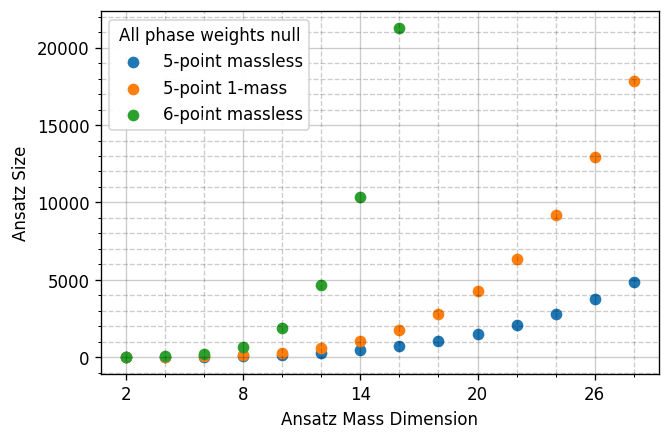
Number of Indep. Functions w/o Subtraction
Technical Interlude: Python Wrapper
$\circ$
Reason 1 : The rational reconstruction, $\mathbb{F}_p \rightarrow \text{Rational Function}$, is much cheaper than numerical evaluations. I want to use
Jupyter for interactive analysis and development.
$\circ$ Reason 2 : Evaluations cost up to 1-2 hours, per phase-space point, per partial amplitude! I need up to ~35k points per partial. (Less for the quark channels, see later.)
We better have some caching!
$\circ$ Pseudo-random squences of phase-space points over $\mathbb{F}_p$ or $\mathbb{Q}_p$ generated using
lips &
pyadic
$\circ$ Custom (for now private) interface to
Caravel, key features:
$\phantom{\circ}\;$ (for Caravel developers see pynta)
$\quad \star$ caching to a SQLite database using
diskcache via Python decorators;
$\quad \star$ distributed computing into a slurm cluster (
use_slurm_cluster=True);
$\quad \star$ functions for IR/UV subtraction, CaravelGraph, and PentagonFunctions parsing;
$\quad \star$ permutations of amplitudes w/o changing call to Caravel.
Polynomial Quotient Rings
$\circ$ Let us start from the polynomial ring of spinor components
$$\displaystyle \kern-50mm S_n = \mathbb{F}\left[|1⟩, [1|, \dots, |n⟩, [n|\right]$$
$\phantom{\circ}$ the field $\mathbb{F}$ can be any of $\mathbb{Q},\mathbb{R},\mathbb{C},\mathbb{F}_p,\mathbb{Q}_p,\dots$
$\circ$ Define the momentum-conservation ideal as
$$
\displaystyle J_{\Lambda_n} = \Big\langle \sum_i |i⟩[i| \Big\rangle_{S_n}
$$
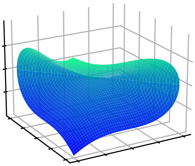
Artist's Impression of $V(J_{\Lambda_n})$
I can't draw in $4n$ dims!
$\phantom{\circ}$ physically, two polynomials $p$ and $q$ are equivalent if $p-q\in J_{\Lambda_n}$
$\circ$ This defines the needed polynomial quotient ring$\kern-4mm\phantom{x}^{\star}$: $\;R_n = S_n / J_{\Lambda_n} $
$r_i(\lambda, \tilde\lambda)$ at $n$-point belong to the Field of Fractions$\kern-4mm\phantom{x}^{\dagger}$ of $R_n$
$\kern-4mm\phantom{x}^\star R_4$ is "weird" (not a UFD), but it proves that polynomial rings are insufficient;
$\;\kern-4mm\phantom{x}^\dagger$ The field of fractions of $R_3$ does not exist.
Prime Ideals & Irreducible Varieties
$\circ$ Let us consider a very simple example (at 4-point)
$\displaystyle \kern-50mm iA_{g^-g^-g^+g^+}^{\text{tree}} = \frac{\langle 12 \rangle^3}{\langle 23 \rangle \langle 34 \rangle \langle 41 \rangle} = \frac{[34]^3}{[12][23][41]} $
$\phantom{\circ}$ is, say, $\langle 23 \rangle$ a pole of this amplitude?
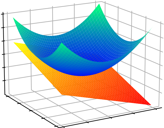
Artist's Impression of $V(\big\langle \langle 23 \rangle\big\rangle_{R_4})$
as the union of two irreducibles
$\circ$ The question is ill posed!
$\phantom{\circ} \langle 23 \rangle$ does not identify an irreducible variety in $R_4$.
$\phantom{\circ}$ Compute $\color{green}\text{primary decompositions}$, such as
$\displaystyle \big\langle \langle 23\rangle \big\rangle_{R_4} = {\color{orange} \big\langle \langle 23\rangle, [14] \big\rangle_{R_4}} \cap {\color{blue} \big\langle \langle 12\rangle, \langle 13 \rangle, \langle 14\rangle, \langle 23\rangle, \langle 24 \rangle, \langle 34 \rangle \big\rangle_{R_4}} $
$\phantom{\circ}$ On the first branch there is a simple pole, on the latter branch the amplitude is regular.
Poles & Zeros $\;\Leftrightarrow\;$ Irreducible Varieties $\;\Leftrightarrow\;$ Prime Ideals
Physics $\kern38mm$ Geometry $\kern38mm$ Algebra
Five-Point Kinematics
$\circ\,$ The rational coefficients take the form
$$
\displaystyle r_i(|i\rangle,[i|) = \frac{\text{Num. poly}(|i\rangle,[i|)}{\text{Denom. poly}(|i\rangle,[i|)} = \frac{\mathcal{N}(|i\rangle,[i|)}{\prod_j D_j^{q_{ij}}(|i\rangle,[i|)}
$$
$\circ\,$ The denominator factors $\mathcal{D}_j$ are conjectured to be restricted to the letters of the symbol alphabet
Abreu, Dormans, Febres Cordero, Ita, Page ('18)
$$
\displaystyle \{\mathcal{D}_{\{1,\dots,35\}}\} = \bigcup_{\sigma \; \in \; \text{Aut}(R_5)} \sigma \circ \big\{ \langle 12 \rangle, \langle 1|2+3|1] \big\} \, , \qquad \text{Aut}(R_5) = \mathcal{P} \times \mathcal{S}_5
$$
$\qquad\color{green}\text{Identical to 1-loop!}$
$\phantom{\circ}$ Non-trivial statement (not proven!): all irreducible polynomials generate prime ideals, @ 5-pt.
$\circ\,$ Advantage of spinor variables:
$1.$ little group covariant LCD (no spurious poles); $\;\;2.$ avoiding parity even/odd split.
$\Rightarrow\;$ fewer and simpler functions to reconstruct compared to Mandelstams or Twistors.
Next we obtain the denomiantor exponents $q_{ij}$.
Least Common Denominator
$\circ\,$ The exponents $q_{ij}$ are given by
$$
\displaystyle \lim_{\mathcal{D}_j \rightarrow 0} r_i = (\mathcal{O}(1) \text{ const.}) \times \mathcal{D}_j^{-q_{ij}}
$$
$\circ\,$ Issue: this can be done for $\mathbb{R}$, $\mathbb{C}$, $\mathbb{Q}_p$ but not $\mathbb{F}_p$ .
$\circ\,$ Solution: univariate Thiele rational interpolation on a line going through $V(\langle \mathcal{D}_j \rangle)$
$$
\displaystyle |i\rangle \rightarrow |i\rangle (t) = |i\rangle + t c_i |\eta\rangle , \qquad |i] \rightarrow |i] \, , \qquad
\text{s.t.} \quad \sum_i c_i |i] = 0
$$
$\circ\,$ After interpolation on the (anti-)holomorphic slice, the rational functions read
$$
\displaystyle r_i(t) = \frac{\text{Poly. }(t)}{\prod_j (t-t_{\mathcal{D}_j})^{q_{ij}}}
$$
where $t_{\mathcal{D}_j}$ is simply the solution to $D_j(t) = 0$. We read off the $q_{ij}$.
Complexity of the Reconstruction
$\circ\,$ Sort the $r_i$ by mass dimension of $\mathcal{N}$ ($\approx$ Ansatz size), pick simplest subset forming a basis $r_{i \in \mathcal{B}}$
Picking a Basis
$\circ\,$ We currently have:
$$
R = r_{i\in \mathcal{B}} M_{ij} h_j \, , \qquad M_{ij} \in \mathbb{Q}
$$
$\phantom{\circ}\,$ with $r_{i\in \mathcal{B}} \subset r_i$, i.e. $M_{ij}$ is in reduced row echelon form, up to a permutation of columns.
$\circ\,$ Basic idea: change basis from a subset of pentagon function coefficients, to linear combinations
$$
\tilde{r}_{i'} = O_{i'i} \, r_{i \in \mathcal{B}} \quad \text{s.t.} \quad \text{rank}(O_{i'i}) = \text{dim(span}_{FF(R_5), \mathbb{Q}}(r_{i}))
$$
$\circ\,$ Key insight:
$$
\text{dim(span}_{FF(R_5), \mathbb{Q}}\left(\lim_{\mathcal{D_j} \rightarrow 0 }r_{i}\right)) \leq \text{dim(span}_{FF(R_5), \mathbb{Q}}(r_{i}))
$$
$\phantom{\circ}\,$ I.e., the pole residues are correlated, build linear combinations that ''remove the overlap''
Correlation of Residues
$\circ\,$ Build Laurent expansions around $t_{\mathcal{D}_k}$
(use same kind of slice as before)
$$
r_{i \in \mathcal{B}} = \sum_{m = 1}^{q_k = \text{max}_i(q_{ik})} \frac{e^k_{im}}{(t-t_{\mathcal{D}_k})^m} + \mathcal{O}((t-t_{\mathcal{D}_k})^0)
$$
$\phantom{\circ}\,$ strictly formal over $\mathbb{F}_p$, but convergent over $\mathbb{Q}_p$ for $(t-t_{\mathcal{D}_k}) \propto p$
$\circ\,$ Repeat for several (anti-)holomorphic slices, build vectors
$$
\vec{e}^k_{im} = (e^k_m)_{ij} = \{ e^k_{im}(\text{slice}_1), \dots, e^k_{im}(\text{slice}_n) \}
$$
$\circ\,$ By Gaussian elimination on the matrix $(e^k_m)_{ij}$ we can partition the space:
$$
\text{span}_{\vec{\mathbb{Q}},\mathbb{Q}}(r_{i \in \mathcal{B}}) = \text{column}_{\vec{\mathbb{Q}},\mathbb{Q}}(\text{Res}(r_{i \in \mathcal{B}}, D_k^m)) \oplus \text{null}_{\vec{\mathbb{Q}},\mathbb{Q}}(\text{Res}(r_{i \in \mathcal{B}}, D_k^m))
$$
Interpretation of $\text{null}_{\vec{\mathbb{Q}},\mathbb{Q}}(\text{Res}(r_{i \in \mathcal{B}}, D_k^m)) \cdot r_{i \in \mathcal{B}}$: functions that do not have a $D_k^m$ singularity
Breadth-First Search
$\circ\,$ If a function $\tilde{r}$ does not have poles $D_{k_1}^{m_1}$ and $D_{k_2}^{m_2}$, then
$$
\tilde{r} \in \text{span}_{FF(R_5),\mathbb{Q}}\Bigg[\Big(\text{null}_{\vec{\mathbb{Q}},\mathbb{Q}}(\text{Res}(r_{i \in \mathcal{B}}, D_{k_1}^{m_1})) \cap \text{null}_{\vec{\mathbb{Q}},\mathbb{Q}}(\text{Res}(r_{i \in \mathcal{B}}, D_{k_2}^{m_2}))\Big)_{i'i} \; \cdot \; r_{i\in \mathcal{B}}\Bigg]
$$
$\circ\,$ Build linear combination that remove as many singularities as possible, without dropping rank
$$
\displaystyle O_{i'i} = \cap_{k, m} \, \text{nulls}_{\vec{\mathbb{Q}},\mathbb{Q}} \qquad \text{(schematically)}
$$
$\circ\,$ This is done by searching a tree of possibilities of which pole gets dropped to which order.
$\phantom{\circ}\,$ Several optimizations required to search an otherwise proibitively large space, naively of size
$$
\prod_k (m_k + 1) \quad \text{with } \; k \;\text{ enumerating } \; D_k^{m_k}
$$
Least Least-Common-Denominator
$\circ$ In other words, we have reshuffled the $r_i$ by linear combinations of the others $r_{j\neq i}$
$\displaystyle \tilde{r}_i = \sum_{j\neq i} O_{ij} r_j + r_i$
$\circ\,$ The rational functions now take the form
$$
\displaystyle \tilde{r}_i(|i\rangle,[i|) = \frac{\tilde{\mathcal{N}}(|i\rangle,[i|)}{\prod_j D_j^{\tilde{q}_{ij}}(|i\rangle,[i|)}
$$
$\phantom{\circ}\,$ where we have minimized $\sum_j \tilde{q}_{ij}$, compared to the $r_i$.
$\circ\,$ This is the closest thing that I am aware of to a Gram–Schmidt procedure for vector spaces over fields that are not number fields, but in this case fields of fractions over polynomial quotient rings.
$\circ\,$ Can we think of this as defining an inner product on the space of rational functions?
$$
O_{ij} \sim \langle r_i | r_j \rangle \qquad \text{(very schematically)}
$$
The Numerator Ansatz
$\circ\,$ The numerator Ansatz takes the form
GDL, Maître ('19)
$\displaystyle \text{Num. poly}(\lambda, \tilde\lambda) = \sum_{\vec \alpha, \vec \beta} c_{(\vec\alpha,\vec\beta)} \prod_{j=1}^n\prod_{i=1}^{j-1} \langle ij\rangle^{\alpha_{ij}} [ij]^{\beta_{ij}}$
$\phantom{\circ}$ subject to constraints on $\vec\alpha,\vec\beta$ due to: 1) mass dimension; 2) little group; 3) linear independence.
$\circ\,$ Construct the Ansatz via the algorithm from Section 2.2 of
GDL, Page ('22)
Linear independence = irreducibility by the Gröbner basis of a specific ideal.
$\circ\,$ Efficient implementation using open-source software only
$\circ\,$ Linear systems solved w/ CUDA over $\mathbb{F}_{2^{31}-1}$ ($t_{\text{solving}} \ll t_{\text{sampling}}$) w/
linac (coming soon-ish)
Spinor-Helicity Results
$\circ$ For the first time with an MHV two-loop five-point amplitude the results for the rational coefficients are compact enough to be present within a paper
https://arxiv.org/pdf/2311.10086.pdf#page=14
$\circ$ The simplification of the basis change is independent of that obtained from partial fraction decompositions, as the latter can still be performed after the former.
$\circ$ Can now study propertities of the amplitude
$\phantom{\circ}$ e.g. no function has a $\text{tr}_5$ singularity, nor a pair of $\langle i | j + k | i]$ in the same denominator.
Quarks from Gluons
$\circ$ Checking whether a rational function belongs to a given vector space
$$
r_{\text{guess}} \stackrel{?}{\in} \text{span}_{FF(R_5), \mathbb{Q}}(r_{i})
$$
$\phantom{\circ}$ is much simpler problem than performing a rational reconstruction!
$\phantom{\circ}$ It only requires as many evaluations as the dimension of the vector space.
$\circ$ The vector space has uniform mass dimension and phase weights
$$
|i⟩ \rightarrow t^{1/2}|i⟩, \; |i] \rightarrow t^{1/2}|i] \quad \forall \; i \quad \text{and} \quad
|i⟩ \rightarrow t|i⟩, \; |i] \rightarrow \frac{1}{t}|i]
$$
$\circ$ Generate guesses for quark functions by re-scaling gluon functions
$$
\tilde{r}^{-}_{73}(q^+,q^-,g^+,g^+,g^-) = \frac{[14]⟨25⟩⟨45⟩}{⟨24⟩[24]⟨34⟩^2} = \frac{⟨14⟩}{⟨24⟩} \underbrace{\frac{[14]⟨25⟩⟨45⟩}{⟨14⟩[24]⟨34⟩^2}}_{r^{--}_{18}(g^+,g^-,g^+,g^+,g^-)}
$$
$\circ$ We obtain most (50% of 2q3g and 90% of 4q1g) quarks functions this way.
Constraints from Poles
Bootstrapping trees (?)
$\circ$ The degree of divergence / vanishing on various surfaces imposes strong constraints, e.g.
$ A^{\text{tree}}_{q^+g^+g^+\bar q^-g^-g^-} = \frac{\mathcal{N(\text{m.d.} = 6\,,\; \text{p.w.} = [-1, 0, 0, 1, 0, 0])}}{\langle 12\rangle\langle 23\rangle\langle 34\rangle [45][56][61]s_{345}}$
$\circ$ Pretend this is un unknown integral coefficient, $\mathcal{N}$ has 143 free parameters.
$\circ$ List the various prime ideal, such as
$ \big\langle \langle 12\rangle, \langle 23\rangle, \langle 13\rangle \big\rangle, \; \big\langle |1\rangle \big\rangle, \; \big\langle \langle 12\rangle, |1+2|3]\big\rangle, \dots$
$\phantom{\circ}$ and impose that $\mathcal{N}$ vanishes to the correct order. We determine it up to an overall constant.
GDL, Page ('22)
$\circ$ Likewise, the ansatz for $A^{\text{tree}}_{g^+g^+g^+ g^-g^-g^-}$ shrinks $1326 \rightarrow 1$, etc..
Effectively, we can compute trees, just from their poles orders.
Note: compared to BCFW there is no information about residues.
Partial Fraction Decompositions
$\circ$ For true integral coefficients, we can't rely on the Ansatz to shrinks to an overall constant.
$\circ$ Partial fraction decompositions (PFDs) are a popular method to tame algebraic complexity.
$\circ$ In my opinion, a PFD algorithm needs
$1.$ to say if two poles $W_a$ and $W_b$ are separable into different fractions;
$2.$ ideally, to answer $(1.)$ without having access to an analytic expression.
$\circ$ Hilbert's nullstellensatz: if $\mathcal{N}$ vanishes on all branches of $\langle W_a, W_b \rangle$, then the PFD is possible$\kern-3mm\phantom{x}^\dagger$.
$\circ$ Generalizing to powers $>\kern-1mm 1$ can be done via symbolic powers and the Zariski-Nagata Theorem.
GDL, Page ('22)
$\circ$ Similarly, generalizing to non-radical ideals requires ring extensions.
Campbell, GDL, Ellis ('22)
Issue: evaluations on singular surfaces are expensive, but are not always needed!
Opportunity: we get more than partial fraction decompositions.
$\kern-4mm\phantom{x}^\dagger$ $\langle W_a, W_b\rangle$ needs to be radical.
Beyond Partial Fractions
$\circ$ $\color{red}\text{Case 0}$: the ideal does $\color{green}\text{not involve denominator factors}$.
E.g. a 6-point function $c_i$ has a pole at $⟨1|2+3|4]$ but not at $⟨4|2+3|1]$,
yet it is regular on the irreducible surface $V(\big\langle ⟨1|2+3|4], ⟨4|2+3|1] \big\rangle)$. Then
$\displaystyle c_i \sim \frac{⟨4|2+3|1]}{⟨1|2+3|4]} + \mathcal{O}(⟨1|2+3|4]^0) \; \text{ instead of } \; c_i \sim \frac{1}{⟨1|2+3|4]} + \mathcal{O}(⟨1|2+3|4]^0)$
$\circ$ $\color{red}\text{Case 1}$: the $\color{green}\text{degree of vanishing is non-uniform}$ across branches, for example:
$\displaystyle \frac{s_{14}-s_{23}}{⟨1|3+4|2]⟨3|1+2|4]}$
has a double pole on the first branch, and a simple pole on the second branch of
$\big\langle⟨1|3+4|2], ⟨3|1+2|4]\big\rangle_{R_6} = \big\langle ⟨13⟩, [24] \big\rangle_{R_6} \cap \big\langle ⟨1|3+4|2], ⟨3|1+2|4], (s_{14}-s_{23})\big\rangle_{R_6}$
$\circ$ $\color{red}\text{Case 2}$: ideal is $\color{green}\text{non-radical}$ (example on last slide)
$\displaystyle \small \kern0mm \sqrt{\big\langle {\color{black}⟨3|1+4|2]}, {\color{black}Δ_{23|14|56}} \big\rangle_{R_6}} = \big\langle {\color{black}⟨3|1+4|2]}, {\color{black}s_{124}-s_{134}} \big\rangle_{R_6} $