Non-planar two-loop QCD
corrections to $\boldsymbol{q\bar q \rightarrow \gamma\gamma\gamma}$:
finite remainders in the spinor-helicity formalism
in collaboration with:
S. Abreu, H. Ita, M. Klinkert, B. Page, V. Sotnikov
based on: arXiv:2305.17056
LoopFest XXI
![]()
![]()
Find these slides at gdelaurentis.github.io/slides/loopfestxxi_june2023
Introduction
State-of-the-Art of
$\boldsymbol{\mathcal{A}^{(2-\textbf{loop})}_{,n}}$
$\circ\,$ $pp\rightarrow \gamma jj$ Badger, Czakon, Hartanto, Moodie, Peraro, Poncelet, Zoia ('23)
$\circ\,$ $pp\rightarrow \gamma\gamma j$ Agarwal, Buccioni, von Manteuffel, Tancredi ('21) Badger, Brønnum-Hansen, Chicherin, Gehrmann, Hartanto, Henn, Marcoli, Moodie, Peraro, Zoia ('21)
$\circ\,$ $pp\rightarrow \gamma\gamma\gamma$ This talk! Abreu, GDL, Ita, Klinkert, Page, Sotnikov ('23);
$\circ\,$ $pp\rightarrow jjj \quad (?)$ Next talk by Federico
Five-point one-mass amplitudes at leading color:
$\circ\,$ $pp\rightarrow Wb\bar b$ Badger, Hartanto, Zoia ('21)
$\circ\,$ $pp\rightarrow Hb\bar b$ Badger, Hartanto, Kryś, Zoia ('21)
$\circ\,$ $pp\rightarrow Wjj$ A bit about this towards the end of this talk! Abreu, Febres Cordero, Ita, Klinkert, Page, Sotnikov ('21);
$\circ\,$ $pp\rightarrow W\gamma j$ Badger, Hartanto, Kryś, Zoia ('22)
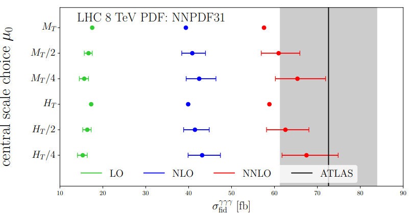
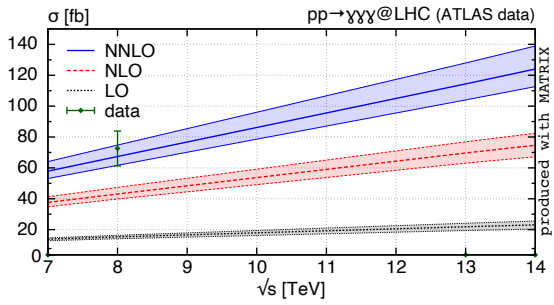
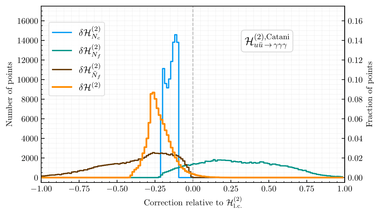
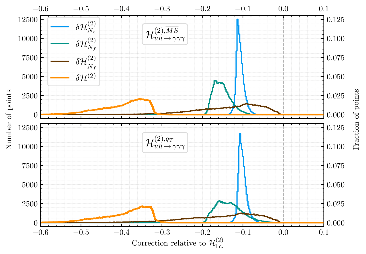
Sizable NNLO Corrections to $\boldsymbol{q\bar q \rightarrow \gamma\gamma\gamma}$
Gauge-Invariant Subamplitudes
| ${\color{green} A^{(2, 0)}_{\,2q3\gamma} }$: | 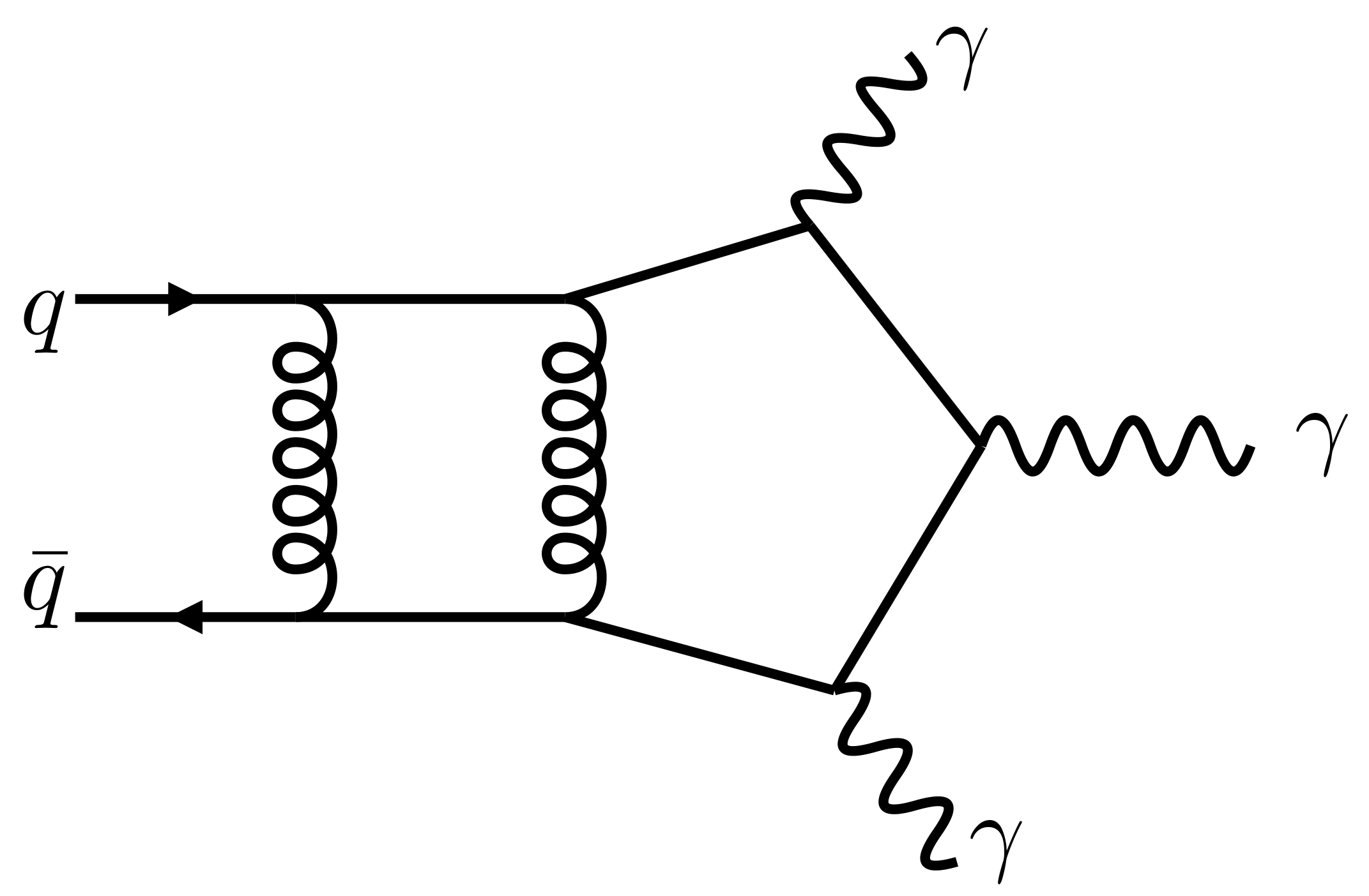 |
${\color{green} A^{(2, N_f)}_{\,2q3\gamma} }$: | 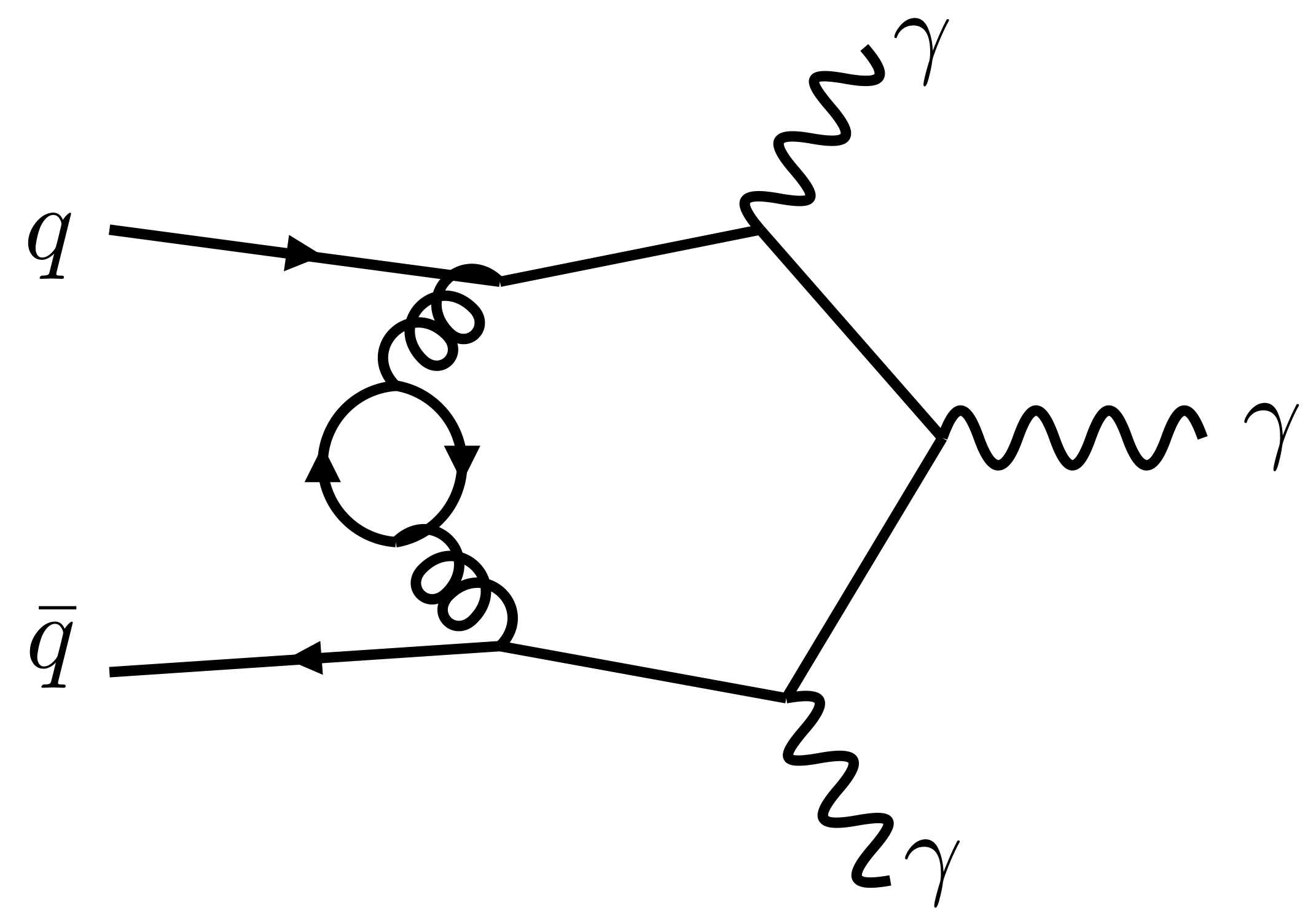 |
Previously known |
| ${\color{red} A^{(2, 1)}_{\,2q3\gamma} }$: | 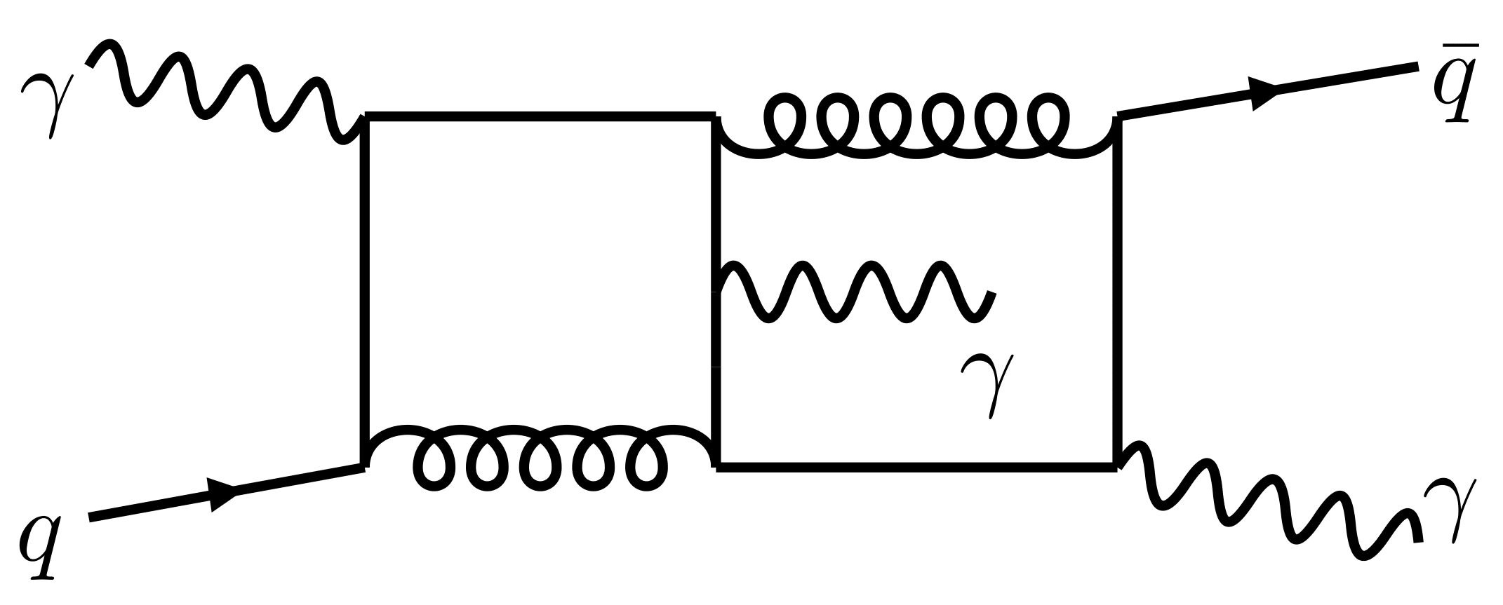 |
${\color{red} A^{(2, \tilde{N}_f)}_{\,2q3\gamma} }$: | 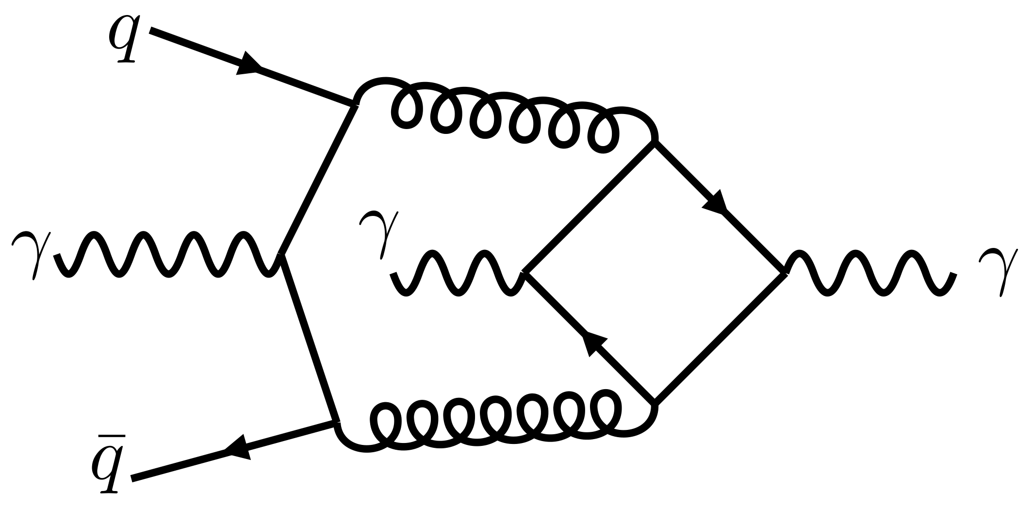 |
New in this work |
Organization
of the Computation
Generalized Unitarity

New Features of the Reduction
Singular + linear algebra.
Finite remainders & the
Rational / Transcendental split
Analytic Reconstruction
The Least Common Denominator
The Numerator Ansatz


Integer programming $\rightarrow$ enumerate sols. $\vec\alpha,\vec\beta$
Perron and Furnon (Google optimization team)
Taming the Algebraic Complexity
$\phantom{\circ\,}$ However, generally $r_{ik} \in \text{span}(r_{j\neq i})$ for some, but not all, $k$. Thus, write:
Towards
Phenomenology
C++ Program
Preview:
$pp\rightarrow Wjj$ Revisited
H. Ita, B. Page, V. Sotnikov
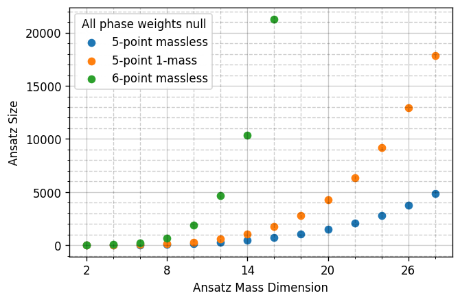
and mass dimension (d):
$\displaystyle \left(\mkern -9mu \begin{pmatrix}\, m(m-3)/2 \, \\ \, d/2 \, \end{pmatrix} \mkern -9mu \right)$
is a lower bound. GDL, Maître ('20)
C++) for evaluation over $\mathbb{F}_p$;
to build 6-point spinor-helicity amplitudes (subject to degree bounds on $|5\rangle,[5|,|6\rangle,[6|$);
| Kinematics | # Poles ($W$) | LCD Ansatz | Partial-Fraction Ansatz | Rational Functions |
| 5-point massless | 30 | 29k | 4k | $\sim$300 KB |
| 5-point 1-mass | >200 | >5M | $\sim$40k | $\sim$25 MB |
for your attention!
markdown, html, revealjs, hugo, mathjax, github
Backup Slides
Absolute Values
on the Rationals
Finite Fields
$\boldsymbol p,$-adic Numbers
Python Packages
pyAdic
Related algorithms, such as rational reconstruction are also implemented.
 from pyadic import ModP
 from fractions import Fraction as Q
 ModP(Q(7, 13), 2147483647)
 <<< 1817101548 % 2147483647
 # Can also go back to rationals
 from pyadic.finite_field import rationalise
 rationalise(ModP(Q(7, 13), 2147483647))
 <<< Fraction(7, 13)
Lips
 from lips import Particles
 from lips.fields.field import Field
 # Random finite field phase space point, arbitrary multiplicity
 multiplicity = 5
 PSP = Particles(multiplicity, field=Field("finite field", 2 ** 31 - 1, 1), seed=0)
 # Evaluate an arbitrary complicated expression
 PSP("(8/3s23⟨24⟩[34])/(⟨15⟩⟨34⟩⟨45⟩⟨4|1+5|4])")
 <<< 683666045 % 2147483647
Spinor Helicity
Representations of the Lorentz group
(Recall: $\mathfrak{so}(1, 3)_\mathbb{C} \sim \mathfrak{su}(2) \times \mathfrak{su}(2)$)| $(j_{-},j_{+})$ | dim. | name | quantum field | kinematic variable |
|---|---|---|---|---|
| (0,0) | 1 | scalar | $h$ | m |
| (0,1/2) | 2 | right-handed Weyl spinor | $\chi_{R\,\alpha}$ | $\lambda_\alpha$ |
| (1/2,0) | 2 | left-handed Weyl spinor | $\chi_L^{\,\dot\alpha}$ | $\bar{\lambda}^{\dot\alpha}$ |
| (1/2,1/2) | 4 | rank-two spinor/four vector | $A^\mu/A^{\dot\alpha\alpha}$ | $P^\mu/P^{\dot\alpha\alpha}$ |
| (1/2,0)$\oplus$(0,1/2) | 4 | bispinor (Dirac spinor) | $\Psi$ | $u, v$ |
Spinor Covariants
Weyl spinors are sufficient for massless particles:
$\text{det}(P^{\dot\alpha\alpha})=m^2 \rightarrow 0 \quad \Longrightarrow \quad P^{\dot\alpha\alpha} = \bar\lambda^{\dot\alpha}\lambda^\alpha$.In terms of 4-momentum components we have:
$$ \lambda\_\alpha=\frac{1}{\sqrt{p^0+p^3}}\begin{pmatrix}p^0+p^3 \\\ p^1+ip^2\end{pmatrix} \, , \;\;\; \lambda^\alpha=\epsilon^{\alpha\beta} \lambda_\beta =\frac{1}{\sqrt{p^0+p^3}}\begin{pmatrix}p^1+ip^2 \\\ -p^0+p^3\end{pmatrix} $$ $\bar\lambda\_{\dot\alpha}=\frac{1}{\sqrt{p^0+p^3}}\begin{pmatrix}p^0+p^3 \\\ p^1-ip^2\end{pmatrix} \, , \;\;\; \bar\lambda^{\dot\alpha}=\epsilon^{\dot\alpha\dot\beta}\bar\lambda_{\dot\beta}=\frac{1}{\sqrt{p^0+p^3}}\begin{pmatrix}p^1-ip^2 \\\ \-p^0+p^3\end{pmatrix}$$$ \bar\lambda\_{\dot\alpha} = (\lambda\_\alpha)^* \quad if \quad p^i \in \mathbb{R}; \quad \quad \bar\lambda\_{\dot\alpha} \neq (\lambda\_\alpha)^* \quad if \quad p^i \in \mathbb{C} $$
Spinor Invariants
The Geometry of Phase Space
based on: GDL, Page (JHEP 12 (2022) 140)
Least Common Denominator Redux
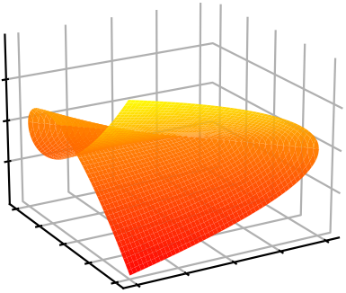
${\color{orange}W_1 = (xy^2 + y^3 - z^2)}$
Multivariate Partial Fractions
${\color{orange}W_1 = (xy^2 + y^3 - z^2)}$
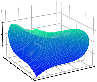
${\color{blue}W_2 = (x^3 + y^3 - z^2)}$
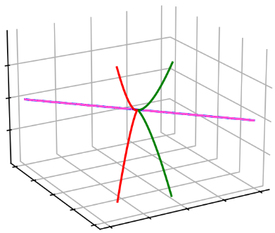
$V(W_1) \cap V(W_2)$