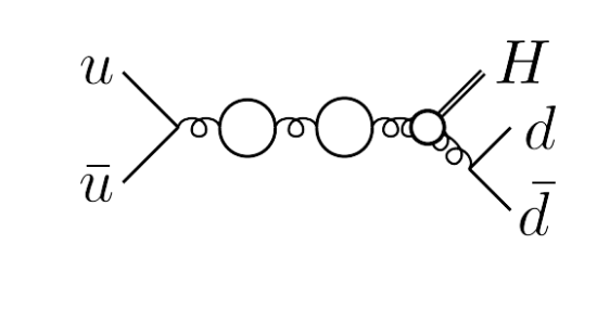
Partial Amplitudes & Finite Remainders
$\circ$ Amplitude (integrands) can be written (for a suitable choice of master integrals) as
$$
\displaystyle A(\lambda, \tilde\lambda, \ell) =
\sum_{\substack{\Gamma,\\ i \in M_\Gamma \cup S_\Gamma}} \, c_{\,\Gamma,i}(\lambda, \tilde\lambda, \epsilon) \, \frac{m_{\Gamma,i}(\lambda\tilde\lambda, \ell)}{\textstyle \prod_{j} \rho_{\,\Gamma,j}(\lambda\tilde\lambda, \ell)} \;\; \xrightarrow[]{\int d^D\ell} \;\; \sum_{\substack{\Gamma,\\ i \in M_\Gamma}} \frac{ \sum_{k=0}^{\text{finite}} \, {\color{red}c^{(k)}_{\,\Gamma, i}}(\lambda, \tilde\lambda) \, \epsilon^k}{\prod_j (\epsilon - a_{ij})} \, {\color{orange}I_{\Gamma, i}}(\lambda\tilde\lambda, \epsilon)
$$
$\circ$ $\Gamma$: topologies $\quad\circ$ $M_\Gamma$: master integrands $\quad\circ$ $S_\Gamma$: surface terms
Abreu, Dormans,
Febres Cordero, Ita
Kraus, Page, Pascual,
Ruf, Sotnikov ('20)

$\circ$ All physical information is contained in the finite remainders, at two loops
Weinzierl ('11)
$$
\underbrace{\mathcal{R}^{(2)}}_{\text{finite remainder}} = \mathcal{A}^{(2)}_R \underbrace{- \quad I^{(1)}\mathcal{A}^{(1)}_R \quad - \quad I^{(2)}\mathcal{A}^{(0)}_R}_{\text{divergent + convention-dependent finite part}} + \mathcal{O}(\epsilon)
$$
Catani ('98)
Becher, Neubert ('09)
Gardi, Magnea ('09)
$\phantom{\circ}$ $\mathcal{A}^{(1)}_R$ to order $\epsilon^2$ is still needed to build $\mathcal{R}^{(2)}$, but there is no real physical reason to reconstruct it.
$$
\textstyle \mathcal{R}(\lambda, \tilde\lambda) = \sum_i \color{red}{r_{i}(\lambda,\tilde\lambda)} \, \color{orange}{G_i(\lambda\tilde\lambda)}
$$
Numerical Computation
$\circ\,$ Direct analytic computations are unfeasible, complexity explodes at intermediate steps.
$\circ\,$ Floating-point evaluations can take hours per point, and lose all precision due to cancellations.
$\circ\,$ The solution is to compute the rational coefficients using finite fields:
$\phantom{\circ}\,$ ordinary arithmetic, but modulo a prime number $p$.
$$
\mathbb{F}_p = \{0,1,\ldots,p-1\}, \qquad
\underbrace{\frac{1}{2} = 4 \pmod 7}_{2\times4=8\equiv1\pmod7}
$$
Exact arithmetic, no rounding errors! Fixed size, no running out of memory!
However, these are not quite the numbers you would want in your Monte Carlo...
$\circ\,$ We have to reconstruct the analytic rational functions from such numerical samples,
$$
\text{Black box} \quad\rightarrow\quad
r_i\big|_{\mathbb{F}_p}
\quad\xrightarrow{\text{reconstruct}}\quad
r_i(\lambda,\tilde\lambda)
\quad\rightarrow\quad
\text{phenomenology}
$$
Goal: compact analytic expressions that are fast and stable to evaluate (in $\mathbb{C}$).
Rational functions of what exactly? A toy example
$\circ$ Manifesting amplitude's gauge and Lorentz invariance, and spin and little-group covariance requires
variables subject to constraints.
$\circ$ Consider polynomials $f, g, h$ in two variables $x, y$. They live in a polynomial ring:
$$
\displaystyle f(x,y), g(x, y), h(x, y) \in \mathbb{Q}[x, y] \, .
$$
$\circ$ Now, restrict them, e.g. on the unit circle $(x^2+y^2-1)$
$$
\displaystyle f(x,y) \approx g(x, y) + h(x, y) (x^2+y^2-1) \, ,
$$
$\phantom{\circ}$ we should consider $f(x,y)$ and $g(x, y)$ as equivalent, for any $h(x,y)$.
$\circ$ The structure is that of a polynomial quotient ring
$$
\displaystyle \mathbb{Q}[x, y] \big/ \big\langle x^2+y^2-1 \big\rangle \\[2mm]
$$
$\phantom{\circ}$ its elements are equivalence classes of polynomials.
$\circ$ $\big\langle x^2+y^2-1 \big\rangle \subset \mathbb{Q}[x, y]$ is an example of an ideal, the infinite set of polynomials
$\phantom{\circ}$ $h(x, y) (x^2+y^2-1)$ that vanishes on the unit circle.
Spinor Component and Invariant Rings
$\circ$ There are two sources of redundancies: kinematic constraints & Schouten/Gram identities.
$\circ$ For $n$-point massless scattering, the covariant quotient ring is
$$
\displaystyle \kern10mm R_{n} = \mathbb{F}\Big[|1⟩_{\alpha}, [1|_{\dot\alpha}, \dots, |n⟩_{\alpha}, [n|_{\dot\alpha} \Big] \Big/ \Big\langle {\textstyle \sum_{i=1}^n} |i\rangle[ i | \Big\rangle
$$
$\phantom{\circ}$ The space has $4n$ dimension subject to $4$ momentum-conservation constraints.
$\circ$ With a single massive leg, e.g. $pp \rightarrow Hjj$, we have $R_{n-1}$ without momentum conservation.
$$
\displaystyle \kern10mm R_{Hjj} = \mathbb{F}\big[|1⟩_{\alpha}, [1|_{\dot\alpha}, |2⟩_{\alpha}, [2|_{\dot\alpha}, |3⟩_{\alpha}, [3|_{\dot\alpha}, |4⟩_{\alpha}, [4|_{\dot\alpha} \big]
$$
$\circ$ Lorentz invariance restricts us to the invariant subring,
generated by spinor brackets:
$$
\displaystyle
\displaystyle R_{Hjj}\supset R_{Hjj}^{SL(2)_L\times SL(2)_R} \cong \mathcal{R}_{Hjj} =
\frac{
\mathbb{F}[\langle ij\rangle,[ij] \;:\; 1\leq i\lt j\leq4]
}{
\big\langle
\langle12\rangle\langle34\rangle-\langle13\rangle\langle24\rangle+\langle14\rangle\langle23\rangle,
\;[12][34]-[13][24]+[14][23]
\big\rangle
}
$$
$\circ$ The rational functions $r_i$ belong to the field of fractions of $R_n$ (or $\mathcal{R}_n \cong R_n^{SL(2)_L\times SL(2)_R}$),
$$
\displaystyle r_i(|i\rangle,[i|) = \frac{\mathcal{N}(|i\rangle,[i|)}{\mathcal{D}(|i\rangle,[i|)} \, , \quad r_i(|i\rangle,[i|) \in \text{Frac}(R_n)
$$
A Tree Example and Denominator Factors
$\circ$ To not make this too abstract, here is the most complex tree amplitude
$$
{A}_g^{(0)}(1^{+}_{g}, 2^{+}_g, 3^{+}_g, 4^{-}_g, \boldsymbol{5}_H) = \Bigg[ \frac{[23]⟨4|2+3|1]^2}{⟨23⟩⟨34⟩[34]s_{234}}+
\frac{[13]⟨23⟩[23]²⟨24⟩⟨34⟩}{⟨12⟩⟨14⟩[14]⟨23⟩⟨34⟩[34]}\Bigg] + \Bigg[ \; \Bigg]_{123456\rightarrow 321456}+\\
\qquad\quad\frac{[13]²⟨4|1+3|2]²}{⟨14⟩[14]⟨34⟩[34]s_{134}}+\frac{[13]²(s_{13}-2s_{123})}{⟨12⟩[14]⟨23⟩[34]}
$$
$\phantom{\circ}$ We need analogous expressions for the MI coefficients.
$\circ$ How do we get them from $\mathbb{F}_p$ evaluations only ? We first need the possible denominators
$\phantom{\circ}$ They are conjectured to be (mostly) related to the letters of the symbol alphabet
Abreu, Dormans, Febres Cordero, Ita, Page ('18)
$\circ$ Surprisingly, they are unchanged from the planar two-loop one-mass amplitudes
$$
\displaystyle \mathcal{D}_{Hjj} = \mathcal{D}_{Vjj} \subset \kern-3mm \bigcup_{\sigma \; \in \; \text{Aut}(R_6)} \sigma \circ \big\{ \langle 12 \rangle, \langle 1|2+3|1], \langle 1|2+3|4], s_{123}, \Delta_{12|34|56}, \underbrace{⟨3|2|5+6|4|3]-⟨2|1|5+6|4|2]}_{\normalsize\text{only new one at two loops!}} \big\}
$$
$\phantom{\circ}$ where $s_{ij} = \langle ij \rangle [ji] $, $s_{ijk} = s_{ij}+s_{ik}+s_{jk} $, $\Delta_{ij|kl|mn}$ is quadratic in the Mandelstams, etc.
Reduced Denominators
$\circ\,$ We can now determine the least common denominators (LCDs),
$$
\displaystyle \mathcal{D} = \prod_j \mathcal{D}_j^{q_{ij}}(|i\rangle,[i|) \, .
$$
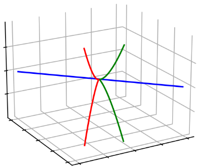
$\phantom{\circ}\,$ Obtain the $q_{ij}$ from a univariate slice $\vec\lambda(t)$, i.e. a 1D curve.
$\circ$ The curve must intersect all varieties $V(\langle \mathcal{D}_j \rangle)$, e.g.
$$
\displaystyle |i\rangle \rightarrow |i\rangle + t a_i |\eta\rangle, \quad [i| \rightarrow [i| + t b_i [\eta|
$$
$\phantom{\circ}\,$ Solve for $a_i, b_i$ such that constraints are satisfied.
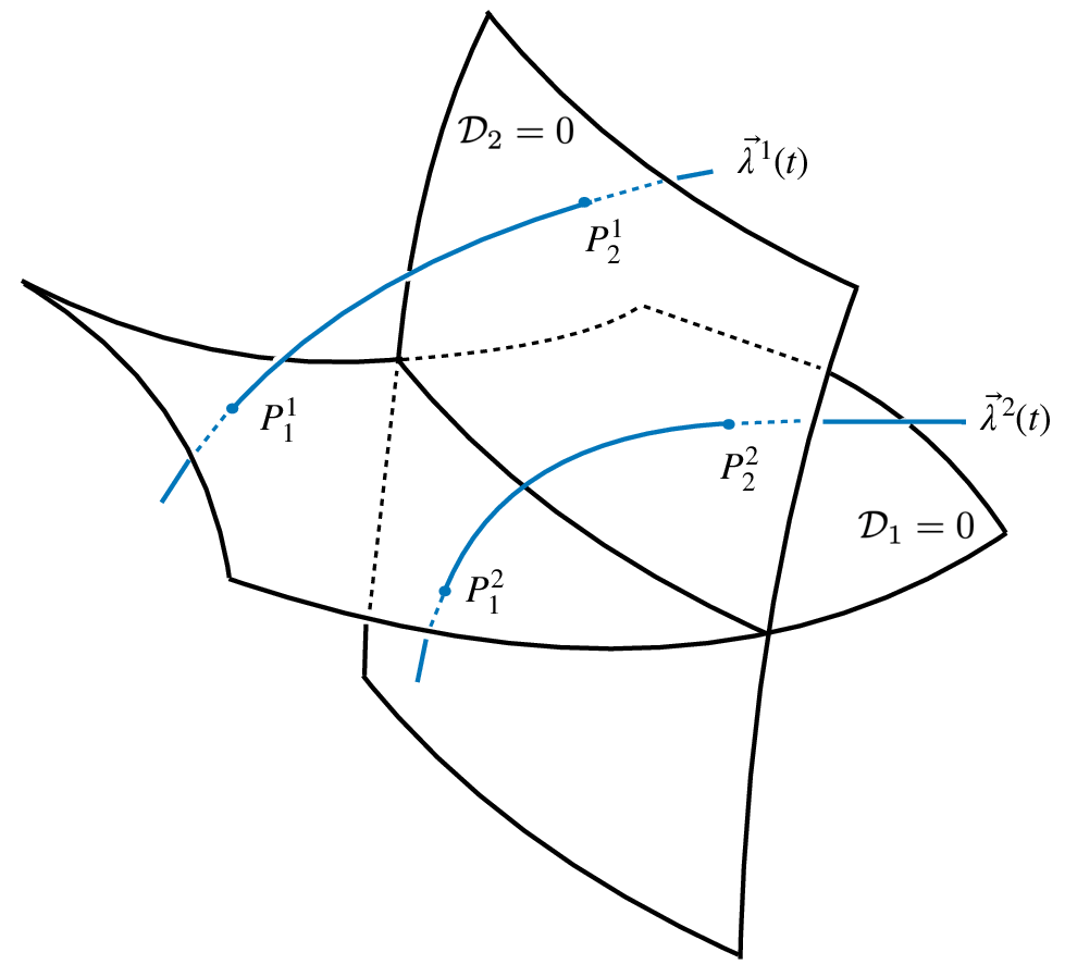
Space has dimension $4n-4$,
$\mathcal{D}_j = 0$ have dimension $4n-5$,
$\vec\lambda(t)$'s have dimension 1.
Poles & Zeros $\;\Leftrightarrow\;$ Irreducible Varieties $\;\Leftrightarrow\;$ Prime Ideals
Physics $\kern24mm$ Geometry $\kern24mm$ Algebra
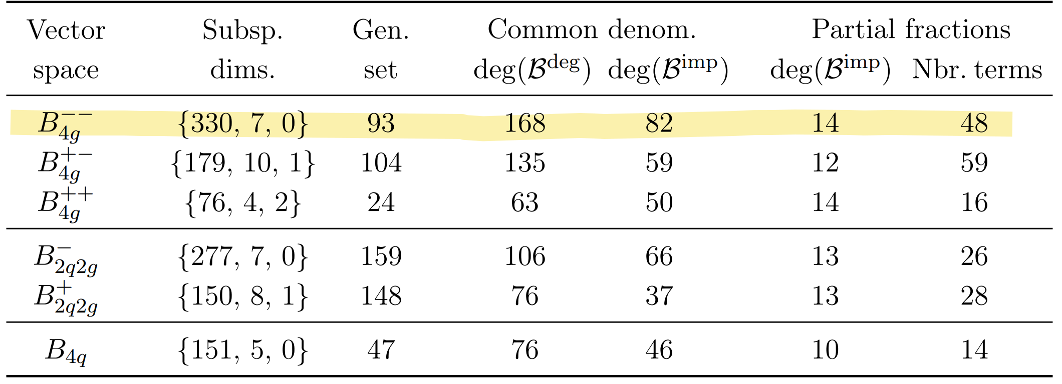
$\phantom{\circ}\,$ For $Hjj$ the most complicated function had a mass dim. ($\approx$ poly. degree) of 168 $\Rightarrow$ 80M parameters
Effect of Basis Change on LCDs
$\circ\,$ Change basis from a subset of the pentagon coefficients $r_{i \in \mathcal{B}}$ to $\mathbb{Q}$-linear combinations $\tilde r$,
$$
R = r_j h_j = r_{i\in \mathcal{B}} M_{ij} h_j = \tilde{r}_{i} \, O_{ii'}M_{i'j} \, h_j \, , \qquad O_{ii'}, M_{i'j}\in \mathbb{Q}
$$
[
6] Abreu, Febres Cordero, Ita, Klinkert, Page, Sotnikov '21
$\circ\,$ For the recent Hjj computation
Basis Change from Laurent Coefficients
$\circ\,$ By Gaussian elimination, partition the space (abusing notation for residue):
$$
\text{span}(r_{i \in \mathcal{B}}) = \underbrace{\text{column}(\text{Res}(r_{i \in \mathcal{B}}, \mathcal{D}_k^m))}_{\text{functions with the singularity}} \;\;\; \oplus \, \underbrace{\text{null}(\text{Res}(r_{i \in \mathcal{B}}, \mathcal{D}_k^m))}_{\text{functions without the singularity}}
$$
$\circ\,$ Search for linear combinations that remove as many singularities as possible (while not dropping rank)
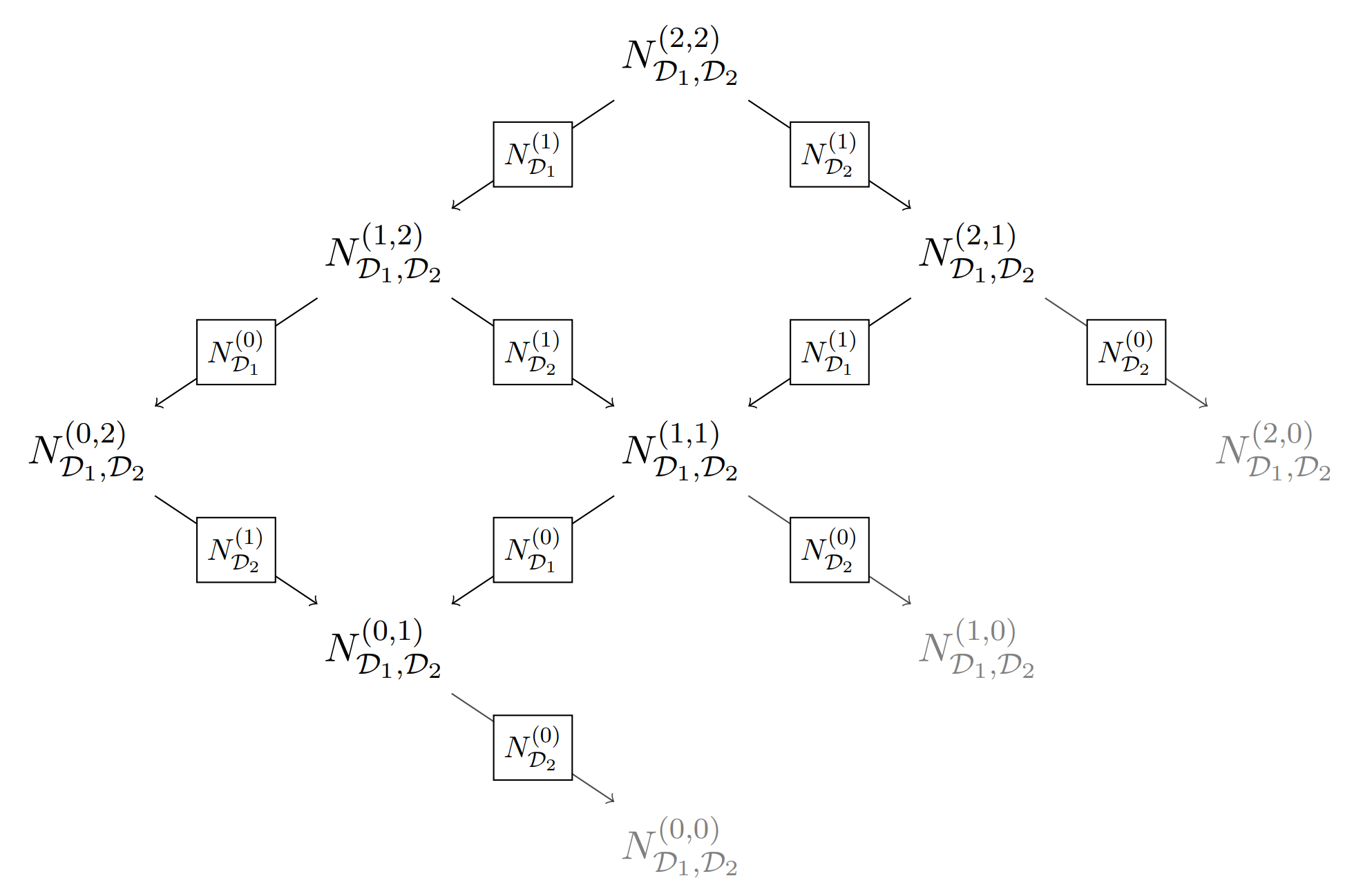
$\phantom{\circ}\,$ $N^{(\text{pole order})}_{\text{denominator factor}}$ denote null-spaces, and arrows denote intersections. Greatest observed breadth $\mathcal{O}(100k)$.
mPFD as Ideal Membership
GDL, Maître ('19)
GDL, Page ('22)
$\circ$ The basis change is still not sufficient. Without knowing $\mathcal{N}$ analytically, we need to answer
$$
\frac{\mathcal{N}}{\mathcal{D}_1\mathcal{D}_2} \stackrel{?}{=}
\frac{\mathcal{N}_2}{\mathcal{D}_1} + \frac{\mathcal{N}_1}{\mathcal{D}_2}
$$
$\circ$ Multivariate partial fraction decompositions follow from varieties where pairs of denominator factors vanish
$$
\frac{\mathcal{N}}{\mathcal{D}_1\mathcal{D}_2} \stackrel{?}{=}
\frac{\mathcal{N}_2}{\mathcal{D}_1} + \frac{\mathcal{N}_1}{\mathcal{D}_2} \; \Longleftrightarrow \; \mathcal{N} \stackrel{?}{\in} \big\langle \mathcal{D}_1, \mathcal{D}_2 \big\rangle \, \text{ i.e. } \; \mathcal{N} \stackrel{?}{=} \mathcal{N}_1 \mathcal{D}_1 + \mathcal{N}_2 \mathcal{D}_2
$$
$$
\langle xy^2 + y^3 - z^2 \rangle + \langle x^3 + y^3 - z^2 \rangle = \langle xy^2 + y^3 - z^2, x^3 + y^3 - z^2 \rangle = \langle 2y^3-z^2, x-y \rangle \cap \langle y^3-z^2, x \rangle \cap \langle z^2, x+y \rangle
$$
$\phantom{\circ}$ This is a primary decomposition. If $\mathcal{N}$ vanishes on all branches, then the partial fraction decomposition exists.
$\circ$ In the end, with a partial fraction decomposition, the largest system we need to solve has $\boldsymbol{\approx 12k}$ unknowns
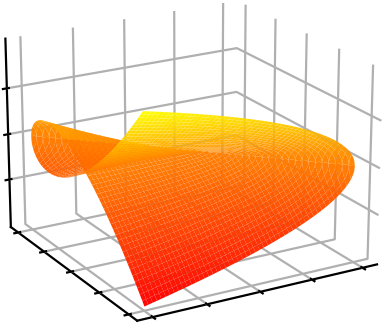
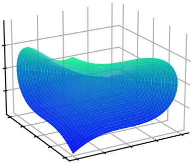
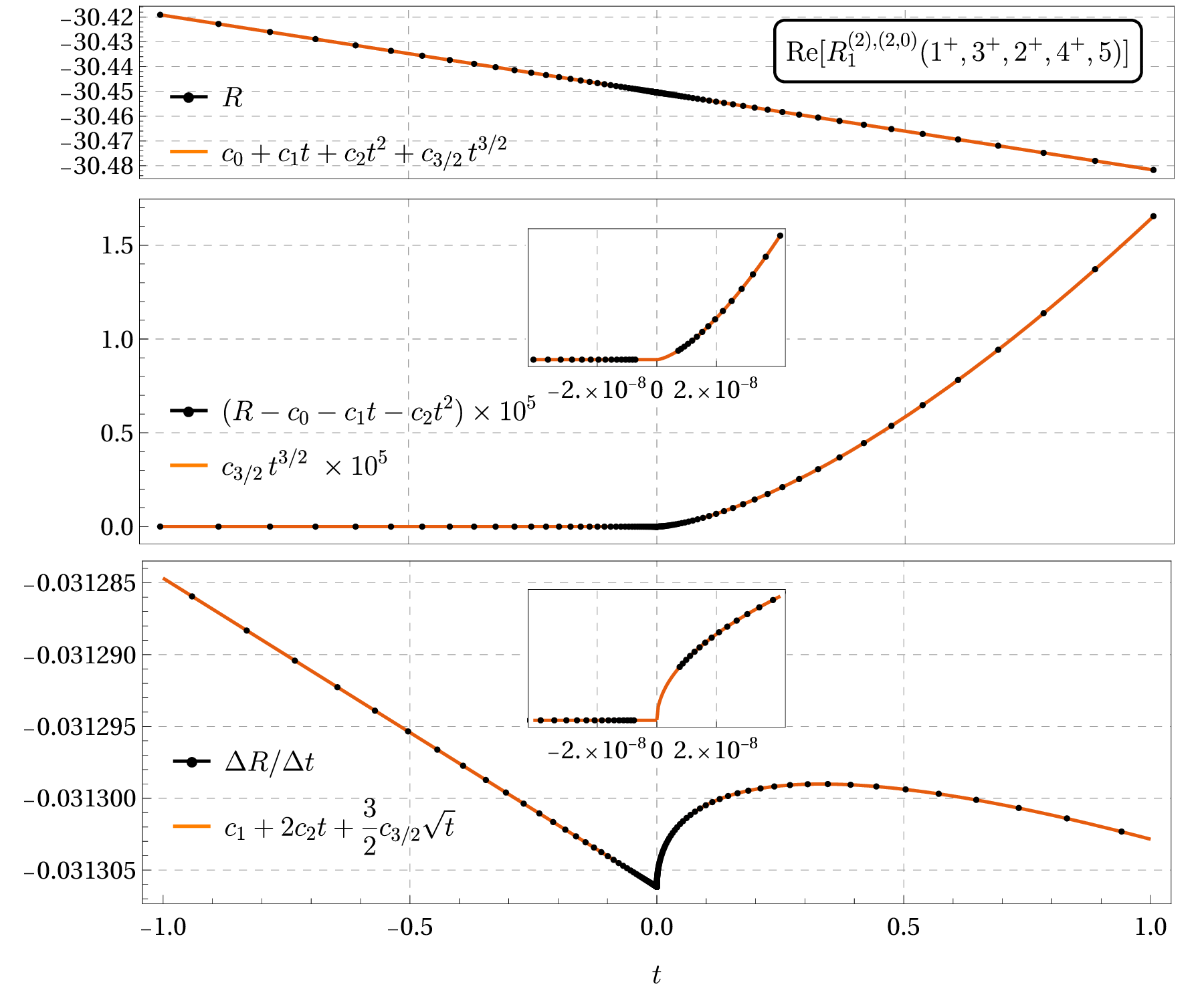
Discontinuity in the second derivative
GDL, Ita, Kuschke, Ruf, Sotnikov
$\circ$ First (?) fully massless pseudo-threshold(?). Cross $\Sigma_5^{(3)}=0 \text{ at } t=0$ ,
$$
\Sigma_5^{(3)} \, = \, \big(s_{12}s_{24}+s_{13}(s_{14}+s_{24})+s_{123}(s_{12}+s_{14})\big)^2-4s_{13}s_{14}s_{123}s_{124} \, .
$$
Bivariate Slice mPFD Algorithm
A partial work-around
$\circ$ Issues: 1) get prim. dec.; 2) sample at codim. two; 3) still need to intersect ideals
$\circ$ Build a bivariate slice (curve) that intersects all varieties $V(\langle \mathcal{D}_i, \mathcal{D}_j \rangle)$, e.g.
$$
\displaystyle |i\rangle \rightarrow |i\rangle + t_1 a_i |\eta\rangle + t_2 b_i |\theta\rangle, \quad [i| \rightarrow [i| + t_1 c_i [\eta| + t_2 d_i [\theta|
$$
$\phantom{\circ}$ Such that for all $t_1, t_2$ momentum is conserved: gives 20 eqs. defining a codim.-10 variety in 24 dims
$\phantom{\circ}$ Pick sol. with syngular.Ideal.points_on_variety, impl. see lips.Particles.bivariate_slice
$\circ$ Reconstruct (Newton-interpolate) the numerators $\mathcal{N}(t_1, t_2)$; this requires $\text{deg}(\mathcal{N}+1)^2$ points.
$\circ$ For each $\mathcal{J}_{ij}^{a_i,a_j} = \big\langle \mathcal{D}_i(t_1, t_2)^{a_i}, \mathcal{D}_j(t_1, t_2)^{a_j} \big\rangle\;$ test $\;\mathcal{N}_i(t_1, t_2) \in \mathcal{J}_{ij}^{a_i,a_j}$
$\circ$ If the test passes, construct the simplified intersection from least common multiples (lcm's)
$$
\begin{equation}
\begin{aligned}\label{eq:RS_merge_generalised}
\mathcal{I}_{\rm s}'&=
\mathcal{I}_{\rm s} \cap_{s} \mathcal{J}_{ij}^{a_ia_j}:=
\big\langle
\mathrm{lcm}(m_1,n_1), \mathrm{lcm}(m_1,n_2), \ldots,
\mathrm{lcm}(m_r,n_1), \mathrm{lcm}(m_r,n_2)
\big\rangle \\
& \kern45mm \mbox{with}\quad
n_1=\mathcal{D}_i(u,v)^{a_i}
\quad\mbox{and}\quad
n_2=\mathcal{D}_j(u,v)^{a_j}\,,
\end{aligned}
\end{equation}
$$
$\phantom{\circ}$ Where $\mathcal{I}_{\rm s}$ starts as the unit ideal, and is otherwise generated by $m_1, \dots, m_r$.
$\circ$ Test $\;\mathcal{N}_i(t_1, t_2) \in \mathcal{I}_{\rm s}'$, if it passes set $\; \mathcal{I}_{\rm s} = \mathcal{I}_{\rm s}'$
Bivariate Slice mPFD Interpretation
$\circ$ In the end we are left with an ideal
$$
\begin{equation}
\mathcal{I}_{\rm s}=\langle m_1(\mathcal{D}),\ldots,m_r(\mathcal{D})\rangle \quad
\mbox{with} \quad \mathcal{N} \in \mathcal{I}_{\rm s} \,.
\end{equation}
$$
$\phantom{\circ}$ whose genreators $m_k$ are monomials in the denominator factors $\mathcal{D}_i$,
$$
\begin{align}
m_k(\mathcal{D}) = \prod_j \mathcal{D}_j^{\hat q_{jk}} \in \mathcal{I}_{\rm s} \quad\mbox{with}\quad k=1,\ldots, r
\end{align}
$$
$\phantom{\circ}$ with powers not exceeding those of the LCD, i.e. no spurious singularities by construction.
$\circ$ We interpret this back in the full multivariate setting as
$$
\mathcal{N} = \sum_{k=1}^{k_{\rm max}} \mathcal{N}_k \, m_k(\mathcal{D} ) \,
$$
$\phantom{\circ}$ and thus the (tentative) multivariate decomposition (Question: how to detect failures before fitting?)
$$
\begin{equation}
\tilde r = \frac{\mathcal{N}}{\prod_j \mathcal{D}_j^{q_j}} =
\sum_{k=1}^{r} \frac{\mathcal{N}_k }{\prod_j \mathcal{D}_j^{q_{jk}}}
\quad\mbox{with} \quad \prod_j \mathcal{D}_j^{q_{jk}} = \frac{\prod_j \mathcal{D}_j^{q_{j}}}{m_k(\mathcal{D})} \, .
\end{equation}
$$
$\circ$ Verify by fitting the ansatz. If it fails, remove some ideals from the intersection.
The Numerator Ansatz
$\circ\,$ The numerator Ansatz takes the form (massless case)
GDL, Maître ('19)
$\displaystyle \text{Num. poly} = \sum_{\vec \alpha, \vec \beta} c_{(\vec\alpha,\vec\beta)} \prod_{j=1}^n\prod_{i=1}^{j-1} \langle ij\rangle^{\alpha_{ij}} [ij]^{\beta_{ij}}$
$\phantom{\circ}$ subject to constraints on $\vec\alpha,\vec\beta$ due to: 1) mass dimension; 2) little group; 3) linear independence.
$\circ\,$ Construct the Ansatz via the algorithm from Section 2.2 of
GDL, Page ('22)
Linear independence = irreducibility by the Gröbner basis of a specific ideal.
$\circ\,$ Efficient implementation using open-source software only
$\circ\,$ Linear systems solved w/ CUDA over $\mathbb{F}_{2^{31}-1}$ ($t_{\text{solving}} \ll t_{\text{sampling}}$) w/
linac (coming soon)
cuda_row_reduce(A, field_characteristic=primes[0], verbose=False) # A is a 2D numpy.ndarray
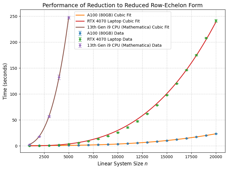
$\circ\,$ Performance on a laptop GPU of approx. 60 CPU cores
$\circ\,$ Performance on a workstation GPU of approx. 600 CPU cores
$\circ\,$ Tested on systems up to 100k equations and unknowns (takes 45 minutes).
 $\;$