Polynomials Modulo Constraints
$\circ$ Manifesting amplitude's gauge and Lorentz invariance, and little-group and spin covariance requires
variables subject to constraints.
$\circ$ Consider polynomials $f, g, h$ in two variables $x, y$. They live in a polynomial ring:
$$
\displaystyle f(x,y), g(x, y), h(x, y) \in \mathbb{Q}[x, y] \, \quad (\text{or more generally} \; \mathbb{F}[x, y]).
$$
$\circ$ Now, localize them, e.g. on the unit circle $(x^2+y^2-1)$
$$
\displaystyle f(x,y) \approx g(x, y) + h(x, y) (x^2+y^2-1) \, ,
$$
$\phantom{\circ}$ we should consider $f(x,y)$ and $g(x, y)$ as equivalent, for any $h(x,y)$.
$\circ$ The structure is that of a polynomial quotient ring
$$
\displaystyle \mathbb{Q}[x, y] \big/ \big\langle x^2+y^2-1 \big\rangle
$$
$\phantom{\circ}$ its elements are equivalence classes of polynomials.
$\circ$ $\big\langle q_1(\underline X), \dots, q_m(\underline X) \big\rangle \subseteq \mathbb{Q}[\underline X]$ is an ideal, the infinite set of polynomials $r_1(\underline X) q_1(\underline X) + \dots $
$\phantom{\circ}$ In this example, the set of polynomials $h(x, y) (x^2+y^2-1)$ that vanish on the unit circle.
Massless Scattering
$\circ$ We have two sources of redundancies: kinematic constraints & Schouten/Gram identities.
$\circ$ For $n$-point massless scattering, the quotient ring is
$$
\displaystyle \kern10mm R_{n} = \mathbb{F}\Big[|1⟩_{\alpha}, [1|_{\dot\alpha}, \dots, |n⟩_{\alpha}, [n|_{\dot\alpha} \Big] \Big/ \Big\langle {\textstyle \sum_{i=1}^n} |i\rangle[ i | \Big\rangle
$$
$\circ$ The "unit circle" is now the codimension $4$ "momentum conservation" variety within a $4n$
$\phantom{\circ}$ dimensional space. On this variety we have equivalence relations such as
$$
\displaystyle \langle 1|2+3|1]=\langle 1|-1-4-5|1]=-\langle 1|4+5|1] \quad \text{in} \quad R_5
$$
$\circ$ The rational functions $r_i$ belong to the field of fractions of $R_n$,
$$
\displaystyle r_i(|i\rangle,[i|) = \frac{\mathcal{N}(|i\rangle,[i|)}{\mathcal{D}(|i\rangle,[i|)} \, , \quad r_i(|i\rangle,[i|) \in \text{Frac}(R_n)
$$
$\circ$ Interesting mathematical observations and open questions:
$\quad\star$ $R_3$ is not an Integral Domain, i.e. it breaks $ab=0 \Rightarrow a = 0 \text{ or } b = 0$ (zero divisors)
$\quad\star$ $R_4$ is not an Unique Factorization Domain (which is why MHV = anti-MHV)
$\quad\star$ Conjecture: $R_{n\geq 5}$ is UFD. For instance, this would imply the denominators $\mathcal{D}$ are unique
$\phantom{\circ}$ Note: all polynomial rings are UFD, so clearly $R_4$ is not equivalent to one, e.g. $\mathbb{F}[s,t]$
Simple Massive Scattering
$\circ$ With a single massive leg, e.g. $pp \rightarrow V(\rightarrow \bar\ell\ell)jj$, we can refer back to massless scattering ($R_6$),
$\phantom{\circ}$ eliminate $p_{V\alpha\dot\alpha}=(5+6)_{\alpha\dot\alpha}$ by mom. conservation and take the decay current to be $[5|\gamma^\mu|6\rangle$
$$
\displaystyle \kern10mm R_{V(\rightarrow\ell\ell')jj} = \mathbb{F}\big[|1⟩_{\alpha}, [1|_{\dot\alpha}, |2⟩_{\alpha}, [2|_{\dot\alpha}, |3⟩_{\alpha}, [3|_{\dot\alpha}, |4⟩_{\alpha}, [4|_{\dot\alpha}, [5|_{\dot\alpha}, |6⟩_{\alpha} \big] \Big/ \big\langle {\textstyle \sum_{i=1}^4} [5|i]\langle i |6\rangle \big\rangle
$$
$\phantom{\circ}$ Assuming we don't partial fraction $s_{1234} = s_{56}=\langle 56\rangle [65]$
to manifest the physical pole $\sqrt{s_{56}}$.
$\phantom{\circ}$ This does not work for multiple massive legs, due to $p_{V_1} \cdot p_{V_2}$ d.o.f.
GDL, Ita, Page, Sotnikov
$\circ$ For $pp \rightarrow HHH$ we use the massive spinor-helicity (or spin-spinor) formalism,
$\phantom{\circ}$ albeit in a very simplified form since scalars have no states.
Shadmi, Weiss Ochirov;
Arkani-Hamed, Huang, Huang;
$$
\displaystyle \kern10mm R_{HHH} = \frac{\mathbb{F}\big[|1⟩_{\alpha}, [1|_{\dot\alpha}, |2⟩_{\alpha}, [2|_{\dot\alpha}, \boldsymbol{3}_{\alpha,\dot\alpha}, \boldsymbol{4}_{\alpha,\dot\alpha}, \boldsymbol{5}_{\alpha,\dot\alpha} \big]}{\big\langle |1\rangle[1|+|2\rangle[2| + \boldsymbol{3}_{\alpha,\dot\alpha} + \boldsymbol{4}_{\alpha,\dot\alpha} + \boldsymbol{5}_{\alpha,\dot\alpha}, \;\, \boldsymbol{3}_{\alpha,\dot\alpha} \boldsymbol{3}^{\dot\alpha,\alpha} - \boldsymbol{4}_{\alpha,\dot\alpha} \boldsymbol{4}^{\dot\alpha,\alpha}, \;\, \boldsymbol{4}_{\alpha,\dot\alpha} \boldsymbol{4}^{\dot\alpha,\alpha}- \boldsymbol{5}_{\alpha,\dot\alpha} \boldsymbol{5}^{\dot\alpha,\alpha} \big\rangle}
$$
$\phantom{\circ}$ where $\boldsymbol{3}_{\alpha,\dot\alpha} \boldsymbol{3}^{\dot\alpha,\alpha} = \boldsymbol{4}_{\alpha,\dot\alpha} \boldsymbol{4}^{\dot\alpha,\alpha} = \boldsymbol{5}_{\alpha,\dot\alpha} \boldsymbol{5}^{\dot\alpha,\alpha} = 2 M_h^2$; $\boldsymbol{3}_{\alpha,\dot\alpha},\boldsymbol{4}_{\alpha,\dot\alpha},\boldsymbol{5}_{\alpha,\dot\alpha}$ are full-rank (unfactorizable).
Campbell, GDL, Ellis
Covariant Q-Rings for Massive Processes
$\circ$ Let's revisit $pp \rightarrow Vjj$, including states in the massive (or spin-spinor) formalism
$$
\displaystyle \kern10mm R_{Vjj} = \mathbb{F}\big[|1⟩_{\alpha}, [1|_{\dot\alpha}, |2⟩_{\alpha}, [2|_{\dot\alpha}, |3⟩_{\alpha}, [3|_{\dot\alpha}, |4⟩_{\alpha}, [4|_{\dot\alpha}, |\boldsymbol 5⟩^J_{\alpha}, [\boldsymbol 5|^I_{\dot\alpha} \big] \Big/ \Big\langle {\textstyle \sum_{i=1}^4} |i]\langle i | + |\boldsymbol 5⟩^I_{\alpha}[\boldsymbol 5|_{I,\dot\alpha} \Big\rangle
$$
GDL, Melnikov, Tresoldi
$$
\displaystyle \text{with} \qquad p_V = |\boldsymbol q^I\rangle [\boldsymbol q_I| = |\boldsymbol q^1\rangle [\boldsymbol q_1| + |\boldsymbol q^2\rangle [\boldsymbol q_2| = |5\rangle [5| + |6\rangle [6|
$$
$$
\displaystyle \varepsilon^{\mu,IJ}_{\boldsymbol 5} = \frac{1}{\sqrt{2}m}[\boldsymbol 5^I|\gamma^\mu|\boldsymbol 5^J\rangle \quad \text{and} \quad \varepsilon^{-} \propto \varepsilon^{11}, \; \varepsilon^{L} \propto \varepsilon^{21} + \varepsilon^{12}, \; \varepsilon^{+} \propto \varepsilon^{22} \quad \text{physical}
$$
Discussion: $\mathcal{A}(1_{\bar q}^{h_1},\,2_g^{h_2},\,3_g^{h_3}\,4_q^{h_4},{\boldsymbol 5}_V^{\pm,L}) = (T^{a_2}T^{a_3})_{i_4}^{\;\bar i_1} A^{IJ}(\dots)\,$ has 3 indep. d.o.f.: $(+++-, ++--, +-+-)$
$\circ$ While $pp \rightarrow ttH$ exposes the full complexity, with multiple massive states
Campbell, GDL, Ellis
$$
\displaystyle \kern10mm R_{ttH} = \frac{\mathbb{F}\big[|1⟩_{\alpha}, [1|_{\dot\alpha}, |2⟩_{\alpha}, [2|_{\dot\alpha}, |\boldsymbol{3}^I⟩_{\alpha}, [\boldsymbol{3}^I|_{\dot\alpha}, |\boldsymbol{4}_J⟩_{\alpha}, [\boldsymbol{4}_J|_{\dot\alpha}, \boldsymbol{5}_{\alpha\dot\alpha} \big]}{\big\langle \sum_{i,I,J} |i\rangle[i|, \langle \boldsymbol{3}|\boldsymbol{3}⟩ +[\boldsymbol{3}|\boldsymbol{3}], \langle \boldsymbol{3}|\boldsymbol{3}⟩-\langle \boldsymbol{4}|\boldsymbol{4}⟩, \langle \boldsymbol{4}|\boldsymbol{4}⟩ +[\boldsymbol{4}|\boldsymbol{4}]\big\rangle}
$$
$\phantom{\circ}$ where $\langle \boldsymbol{3}^I|\boldsymbol{3}^J⟩=m\epsilon^{JI} \text{ and } [\boldsymbol{3}^I|\boldsymbol{3}^J]=\bar{m}\epsilon^{IJ}$; we are setting $m=\bar{m}$ and the tops on-shell.
$\circ$ !Overparametrisation Warning! Remember the map to massless case,
Conde, Marzolla;
Conde, Joung, Mkrtchyan
$$
\displaystyle 1 \rightarrow 1, 2 \rightarrow 2, \boldsymbol{3} \rightarrow 3+4, \boldsymbol{4} \rightarrow 5+6, \boldsymbol{5} \rightarrow 7+8
$$
Examples of Trees
$\circ$ To not make this too abstract, we are after expressions like these, but for the MI coefficients.
$\circ$ For $Vjj$ there are 5 amplitudes (showing 3)
$$
{A}_g^{(0)}(1^{+}_\bar{q}, 2^{+}_g, 3^{+}_g, 4^{-}_q, 5^{+}_\bar{\ell}, 6^{-}_\ell) = \frac{⟨46⟩^2}{⟨12⟩⟨23⟩⟨34⟩⟨65⟩} \, \Rightarrow {A}_g^{(0),{IJ}}(1^{+}_\bar{q}, 2^{+}_g, 3^{+}_g, 4^{-}_q, {\boldsymbol 5}) = \frac{⟨4|\boldsymbol 5|\boldsymbol 5^I]⟨\boldsymbol 5^J 4⟩}{⟨12⟩⟨23⟩⟨34⟩s_{\boldsymbol 5}} , \\[6mm]
{A}_g^{(0)}(1^{+}_\bar{q}, 2^{+}_g, 3^{-}_g, 4^{-}_q, 5^{+}_\bar{\ell}, 6^{-}_\ell) = \frac{⟨13⟩⟨3|1+2|5]^2}{⟨12⟩⟨23⟩[65]⟨1|2+3|4]s_{123}} \; + \; (123456\rightarrow \overline{432165}) \, , \\[6mm]
{A}_q^{(0)}(1^{+}_\bar{q}, 2^{+}_{q'}, 3^{+}_{\bar{q}'}, 4^{-}_q, 5^{+}_\bar{\ell}, 6^{-}_\ell) = -\frac{[12]⟨46⟩⟨3|1+2|5]}{⟨23⟩[23]⟨56⟩[56]s_{123}}+(123456\rightarrow 156423)\phantom{+}
$$
$\circ$ For $q\bar{q}\rightarrow t\bar{t}H$ there is only a single amplitude
$$
{A}_{ttH}^{(0)}(1^{+}_q, 2^{-}_\bar{q}, 3_t, 4_\bar{t}, 5_H)^I_J = \frac{⟨2|𝟑|1]⟨𝟑^I𝟒_J⟩-[𝟑^I1][1𝟒_J]⟨12⟩}{s_{12}(s_{12𝟑}-m_t²)} +
(12345\rightarrow\overline{21345},12435,\overline{21435})
$$
$\phantom{\circ}$ where for clarity I have not suppressed the spin indices. Symmetries are made manifest.
$\phantom{\circ}$ Note: The amplitude is spin covariant, just like it is little group covariant!
$\phantom{\circ} \kern7mm$ We need only obtain a single choice, say $I=J=1$, the other follows.
Spinor Alphabets
$\circ$ We can always factorize a polynomial into products of irreducible factors, to some powers
$$
\displaystyle r_i(|i\rangle,[i|) = \frac{\mathcal{N}(|i\rangle,[i|)}{\prod_j \mathcal{D}_j^{q_{ij}}(|i\rangle,[i|)} % \, , \quad r_i(|i\rangle,[i|) \in \text{Frac}(R_n)
$$
$\phantom{\circ}$ For the numerators this is generally not particularly useful (when in least common denominator form)
$\phantom{\circ}$ The denominator factors $\mathcal{D}_j$ are conjectured to be (mostly) related to the letters of the symbol alphabet
Abreu, Dormans, Febres Cordero, Ita, Page ('18)
$\circ$ Convert your alphabet from independent Mandelstam invariants to redudant spinors brackets
From work in progress with S. Abreu, X. Liu, P.F. Monni
Mandelstam letters
$s_{12}$
$s_{123}$
$s_{12} - s_{123} - s_{345} + s_{45}$
$-s_{12} + s_{123}$
$s_{12}(s_{123} - s_{56}) - s_{123}(s_{123} + s_{34} - s_{56})$
$\displaystyle\frac{
s_{12}\left(s_{16}(s_{23} - s_{234})s_{34} + s_{23}^{2}(\cdots) + \cdots\right) + s_{123}(\cdots) + s_{23}(\cdots)
}{
\sqrt{(-s_{12} + s_{123} - s_{23})^2\cdots}
}$
$\Rightarrow$
Spinor letters
$\langle 1\,2\rangle[1\,2]$
$s_{123}$
$\langle 3\,|\,6\rangle[3\,|\,6]$
$\langle 3\,|\,1{+}2\,|\,3]$
$\langle 3\,|\,1{+}2\,|\,4]\langle 4\,|\,1{+}2\,|\,3]$
$\operatorname{tr}_5(2,3,4,5)$
$\circ$ Factorization and extra chiral cancellations are key for simplification in gauge amplitudes
What to do with square roots?
$\circ$ The transcendental basis is pure up to some square roots
$$
\displaystyle \mathcal{R}(\lambda, \tilde\lambda) = \sum_i \color{red}{r_{i}(\lambda,\tilde\lambda)} \, \color{orange}{G_i(\lambda\tilde\lambda)} \color{black} \; , \qquad G_i = h_i \quad \text{or} \quad G_i = \frac{h_i}{\sqrt{q}}
$$
$\phantom{\circ}$ with $h_i$ pure and $q$ irreducible polynomials in Mandelstams
$\circ$ Distinguish 3 cases for $\sqrt{q} = \sqrt{\Delta_3}, \sqrt{\Delta_5}, \sqrt{\Sigma_5}$
$\quad 1.$ $\sqrt{q} = \sqrt{\Delta_3}$ is the boring case, leave it unchanged, here $\lim_{q\rightarrow 0} h_i = \sqrt{q}$,
$$
G_i \rightarrow \frac{h_i}{\sqrt{\Delta_3}}
$$
$\quad 2.$ $\sqrt{q} = \sqrt{\Delta_5}$ is rational in spinors, $\sqrt{\Delta_5} = \pm \text{tr}(\gamma^5p_1p_2p_3p_4) = \pm ([1|2|3|4|1\rangle-\langle1|2|3|4|1])$,
$$
G_i \rightarrow \frac{\text{tr}_5}{\sqrt{\Delta_5}} h_i = \text{sign}\big(\text{Im}(\text{tr}_5)\big) h_i
$$
$\quad 3.$ $\sqrt{q} = \sqrt{\Sigma_5}$, the rational coefficient vanishes linearly in $\lim_{q\rightarrow 0}$,
$$
G_i \rightarrow \sqrt{\Sigma_5} \, h_i
$$
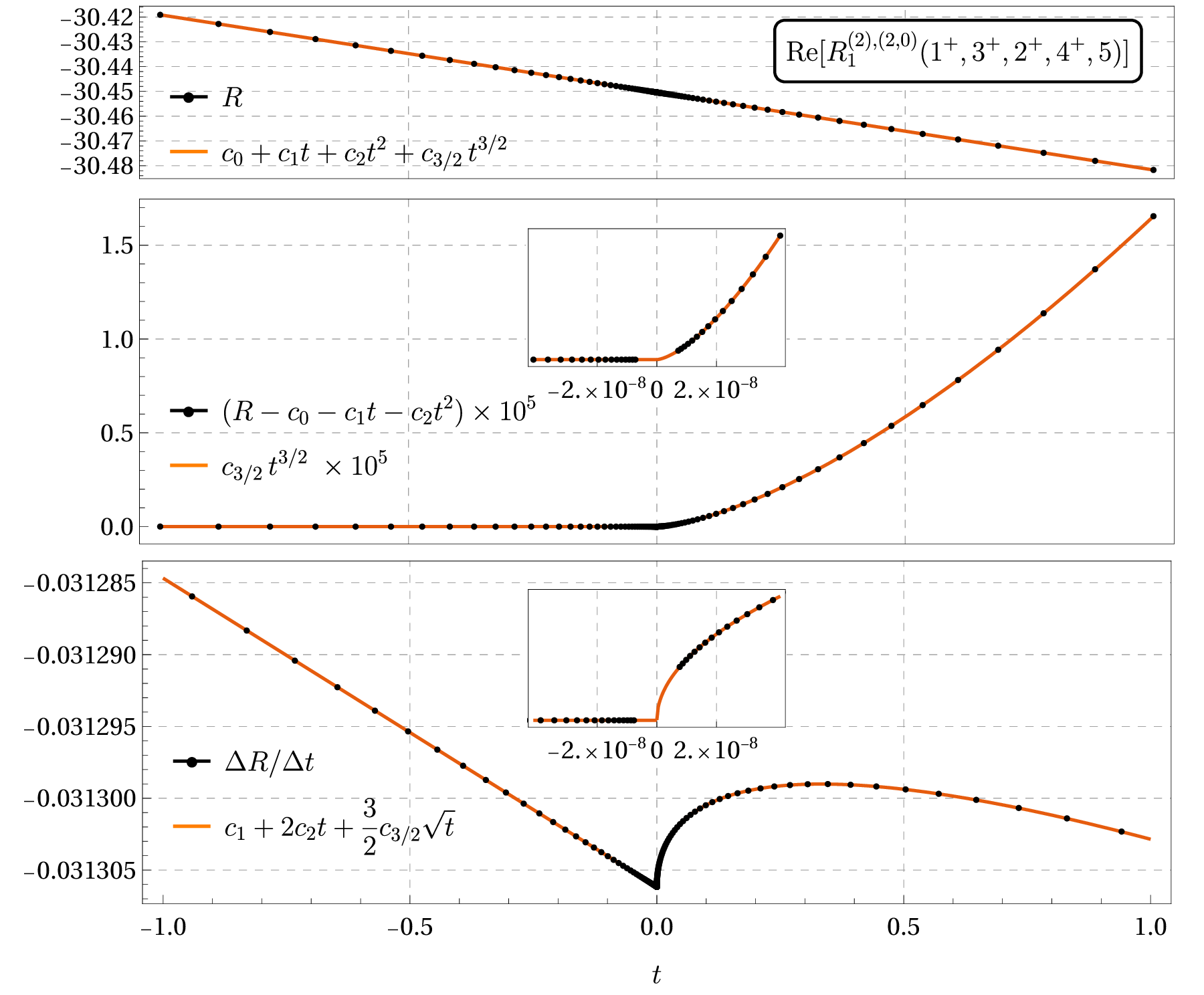
Discontinuity in the second derivative remainder
GDL, Ita, Kuschke, Ruf, Sotnikov
$\circ$ First (?) fully massless pseudo-threshold(?). Cross $\Sigma_5^{(3)}=0 \text{ at } t=0$ ,
$$
\Sigma_5^{(3)} \, = \, \big(s_{12}s_{24}+s_{13}(s_{14}+s_{24})+s_{123}(s_{12}+s_{14})\big)^2-4s_{13}s_{14}s_{123}s_{124} \, .
$$
Least Common Denominator
(Geometry at codimension one)
Least Common Denominator
$\circ\,$ We can now determine the least common denominators (LCDs),
$$
\displaystyle \mathcal{D} = \prod_j \mathcal{D}_j^{q_{ij}}(|i\rangle,[i|) \, .
$$
$\phantom{\circ}\,$ Obtain the $q_{ij}$ from a univariate slice $\vec\lambda(t)$, i.e. a 1D curve.
$\circ$ The curve must intersect all varieties $V(\langle \mathcal{D}_j \rangle)$, e.g.
$$
\displaystyle |i\rangle \rightarrow |i\rangle + t a_i |\eta\rangle, \quad [i| \rightarrow [i| + t b_i [\eta|
$$
$\phantom{\circ}\,$ Solve for $a_i, b_i$ such that constraints are satisfied.
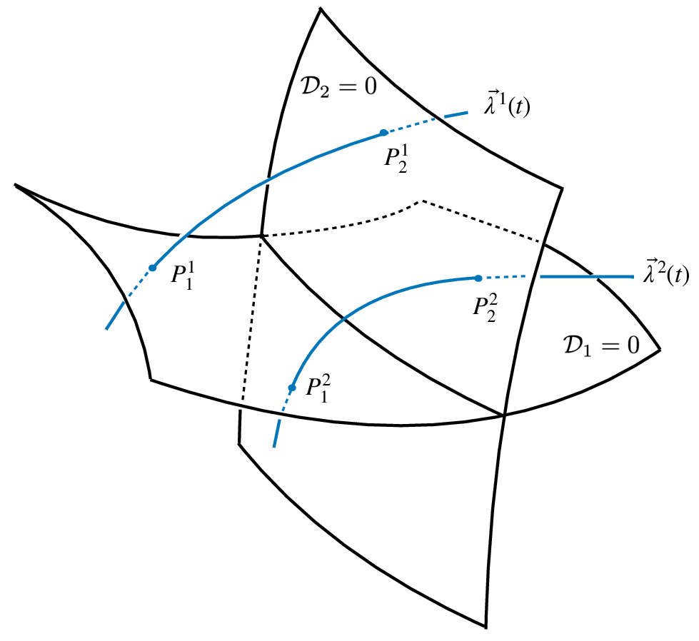
Space has dimension $4n-4$,
$\mathcal{D}_j = 0$ have dimension $4n-5$,
$\vec\lambda(t)$'s have dimension 1.
Poles & Zeros $\;\Leftrightarrow\;$ Irreducible Varieties $\;\Leftrightarrow\;$ Prime Ideals
Physics $\kern18mm$ Geometry $\kern18mm$ Algebra
Open-Source Implementation
$\circ\,$ Example: determine the LCDs of a vector of finite-remainder coefficients.
from antares.core.numerical_methods import tensor_function
from lips import Particles
oTF = tensor_function(lambda oPs: numpy.array(
    [coeff for coeff, monom in amps['qbpqmqbpqm_2L_Nc2_Nf0'].finite_remainder(oPs)] +
    [coeff for coeff, monom in amps['qbpqmqbpqm_2L_Nc1_Nf1'].finite_remainder(oPs)] +
    ....
))
oTF.multiplicity = 6
oTF.__name__ = '4q1h_mhv'  # qbar+ q- qbar+ q- H, through two loops

oSlice = Particles(6, field=Field("finite field", 2 ** 31 - 1, 1), seed=0)
oSlice.univariate_slice(algorithm='covariant', seed=0)

lTermsLCD = oTF.get_lcds(oSlice, verbose=True)
lTermsLCD[:5]
[
  Terms("""+(1)/(⟨1|2⟩[1|2]⟨3|4⟩[3|4]⟨1|3+4|1]⟨2|3+4|2]⟨3|1+2|3]⟨4|1+2|4])"""),
  Terms("""+(1)/(⟨1|2⟩[1|2]⟨1|3⟩[2|4]⟨3|4⟩[3|4]⟨1|2+3|1]⟨4|2+3|4])"""),
  Terms("""+(1[1|3])/(⟨1|3⟩⟨1|2+3|1]⟨3|1+2|3]²)"""),
  Terms("""+(1⟨2|4⟩)/([2|4]⟨2|3+4|2]²⟨4|2+3|4])"""),
  ...
]
LCD Factors / Kinematic Poles / Letters
$\circ\,$ The irreducible denominator factors $\mathcal{D}_j \text{ for } Vjj$ (modding out by permutation orbits) read
$$
\displaystyle \mathcal{D}_{Hjj} = \mathcal{D}_{Vjj} \subset \kern-3mm \bigcup_{\sigma \; \in \; \text{Aut}(R_6)} \sigma \circ \big\{ \langle 12 \rangle, \langle 1|2+3|1], \langle 1|2+3|4], s_{123}, \Delta_{12|34|56}, \underbrace{⟨3|2|5+6|4|3]-⟨2|1|5+6|4|2]}_{\normalsize\text{only new one at two loops!}} \big\}
$$
$\circ\,$ For $t\bar{t}H$ (at one-loop), they read
$$
\displaystyle \kern-10mm \mathcal{D}_{ttH} = \big\{ \langle 12 \rangle, [12], s_{123}, \dots, (s_{123}-m^2), \langle 1|\boldsymbol{3}|1], \dots, \\[2mm]
\kern30mm \langle 1|\boldsymbol{3}|\boldsymbol{4}| 2 \rangle, \dots, \langle 1|\boldsymbol{3}|1+2|\boldsymbol{4}| 2], \dots, \Delta_{12|34|5}, \dots \Delta_{12|3|4|5} \big\}
$$
$\phantom{\circ}\,$ note that there is no dependence on the top states (this looks like 3 massive scalars).
$\circ\,$ For $HHH$ (at one-loop), they are
$$
\small
\begin{gathered}
\mathcal{D}_{HHH} = \big\{
⟨1|2⟩, [1|2], ⟨2|𝟓|1], ⟨2|𝟒|1], ⟨2|𝟑|1], ⟨1|𝟑|2], [1|𝟑|𝟓|1], ⟨1|𝟑|𝟓|1⟩, ⟨1|𝟓|𝟒|2⟩, [2|𝟒|𝟓|1], Δ_{12|𝟑|𝟒|𝟓}, \\
⟨2|𝟑|𝟒|𝟓|1], ⟨1|𝟓|𝟒|𝟑|2], ⟨1|2⟩[1|2]⟨1|𝟓|𝟒|𝟑|2]⟨2|𝟑|𝟒|𝟓|1]+m_t^2\text{tr}_5(1|2|𝟑|𝟒)^2, \\
⟨1|𝟑|2]⟨2|𝟒|𝟓|1⟩[1|𝟑|2⟩[2|𝟒|𝟓|1]+m_t^2\text{tr}_5(1|2|𝟑|𝟒)^2
\big\}
\end{gathered}
$$
$\circ\,$ Challenge: in LCD form the numerators are intractably complicated.
$\phantom{\circ}\,$ E.g. for $Vjj$ the most complicated function had a mass dim. ($\approx$ poly. degree) of 114 $\Rightarrow$ 25M parameters
$\phantom{\circ}\,\qquad$ (and non-trivial little group weights $\{3, -12, 12, -3, -1, 1\}$ due to chiral cancellations!)
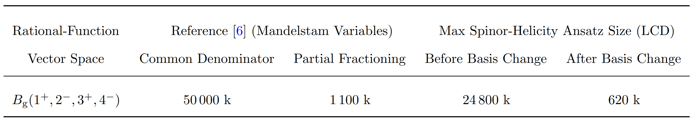
$\phantom{\circ}\,$ For $Hjj$ the most complicated function had a mass dim. ($\approx$ poly. degree) of 168 $\Rightarrow$ 80M parameters
Effect of Basis Change on LCDs
$\circ\,$ Change basis from a subset of the pentagon coefficients $r_{i \in \mathcal{B}}$ to $\mathbb{Q}$-linear combinations $\tilde r$,
$$
R = r_j h_j = r_{i\in \mathcal{B}} M_{ij} h_j = \tilde{r}_{i} \, O_{ii'}M_{i'j} \, h_j \, , \qquad O_{ii'}, M_{i'j}\in \mathbb{Q}
$$
[
6] Abreu, Febres Cordero, Ita, Klinkert, Page, Sotnikov '21
$\circ\,$ For the recent Hjj computation
Basis Change from Laurent Coefficients
$\circ\,$ By Gaussian elimination, partition the space (abusing notation for residue):
$$
\text{span}(r_{i \in \mathcal{B}}) = \underbrace{\text{column}(\text{Res}(r_{i \in \mathcal{B}}, \mathcal{D}_k^m))}_{\text{functions with the singularity}} \;\;\; \oplus \, \underbrace{\text{null}(\text{Res}(r_{i \in \mathcal{B}}, \mathcal{D}_k^m))}_{\text{functions without the singularity}}
$$
$\circ\,$ Search for linear combinations that remove as many singularities as possible (while not dropping rank)
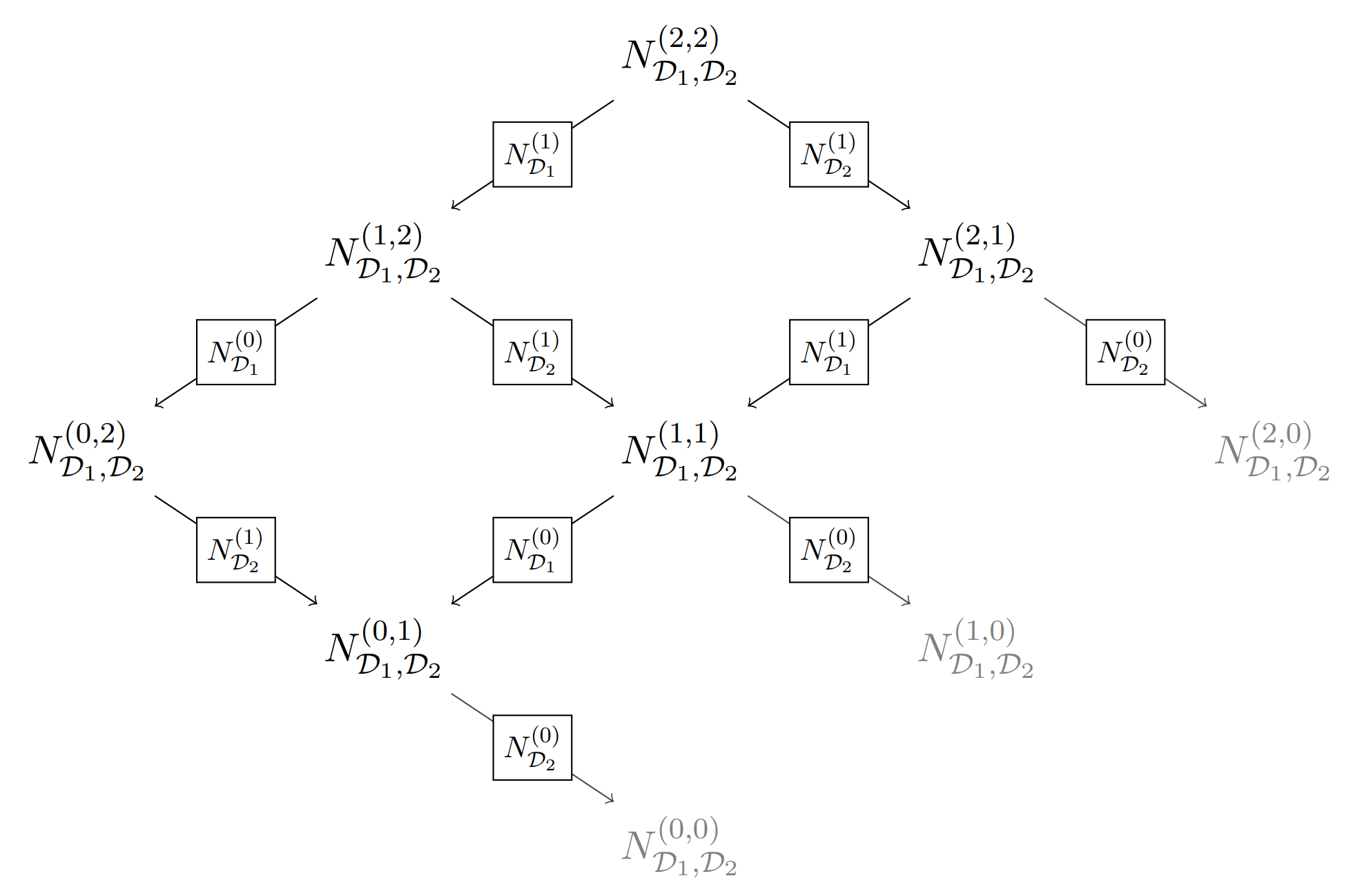
$\phantom{\circ}\,$ $N^{(\text{pole order})}_{\text{denominator factor}}$ denote null-spaces, and arrows denote intersections. Greated observed breadth $\mathcal{O}(100k)$.
$p\kern0.5mm$-adic numbers
$\circ$ You may be familiar with finite field (integers modulo a prime)
von Manteuffel, Schabinger `14;$\;$ Peraro `16
$$
\displaystyle a \in \mathbb{F}_p : a \in \{0, \dots, p -1\} \; \text{ with } \; \{+, -, \times, \div\}
$$
$\phantom{\circ}$ Limits (and calculus) are not well defined in $\mathbb{F}_p$. We can make things zero, but not small:
$$
\displaystyle |a|_0 = 0 \; \text{if} \; a = 0 \; \text{else} \; 1 \quad \text{a.k.a. the trivial absolute value.}
$$
$\circ$ There exists just one more absolute value on the rationals, the $p$-adic absolute value.
Ostrowski's theorem 1916
$\circ$ Let's start from $p$-adic integers, instead of working modulo $p$, expand in powers of $p$
$$
\displaystyle a \in \mathbb{Z}_p : a_0 p^0 + a_1 p^1 + a_2 p^2 + \dots + \mathcal{O}(p^n)
$$
$\phantom{\circ}$ In some sense we are correcting the finite field result with more (subleading) information.
$\circ$ $p$-adic numbers $\mathbb{Q}_p$ allow for negative powers of $p$, (would be division by zero in $\mathbb{F}_p$!)
$$
\displaystyle a \in \mathbb{Q}_p : a_{-\nu} p^{-\nu} + \dots + a_0 + a_1 p^1 + \dots + \mathcal{O}(p^n)
$$
GDL, Page `22
$\circ$ The $p$-adic absolute value is defined as $|a|_p = p^\nu$.
$\phantom{\circ}$ Think of $p$ as a small quantity, $\epsilon$, (by $|\,|_p$) even if it is a large prime (by the real abs. $|\,|_\infty$).
Laurent Series or p(z)-adic expansion
$\circ\,$ With $p$-adic numbers this would be straight forward, set $\mathcal{D}_j\propto p$ and evaluate the function
$$
r_{i\in \mathcal{B}} = \sum_{m = 1}^{\text{max}_i(q_{ik})} \frac{e^k_{im}}{p^m} + \mathcal{O}(p^0) \text{ is a number in } \mathbb{Q}_p
$$
$\phantom{\circ}\,$ See Particles._singular_variety or Ideal.point_on_variety to generate the configuration
$\circ\,$ We can't do this with only finite fields. Instead, build Laurent expansions around $t_{\mathcal{D}_k}$ (use more slices)
$$
r_{i \in \mathcal{B}} = \sum_{m = 1}^{\text{max}_i(q_{ik})} \frac{e^k_{im}}{(t-t_{\mathcal{D}_k})^m} + \mathcal{O}((t-t_{\mathcal{D}_k})^0)
$$
$\phantom{\circ}\,$ strictly formal over $\mathbb{F}_p$, but convergent over $\mathbb{Q}_p$ for $(t-t_{\mathcal{D}_k}) \propto p$
$\circ\,$ What if the letter does not have a factor linear in $t$? E.g.
$$
r_{i \in \mathcal{B}} = \sum_{m = 1}^{\text{max}_i(q_{ik})} \frac{c^k_{im} t + d^k_{im}}{(t^2+a_kt+b_k)^m} + \mathcal{O}((t^2+a_kt+b_k)^0)
$$
see also Fontana, Peraro ('23)
$\circ\,$ From these coefficients, build null spaces used in the search for simple functions
$$
\text{null}(\text{Res}(r_{i \in \mathcal{B}}, \mathcal{D}_k^m))_{ij} \text{ from } \text{ rref } (d^k_{m})_{i,\text{slice}_j}
$$
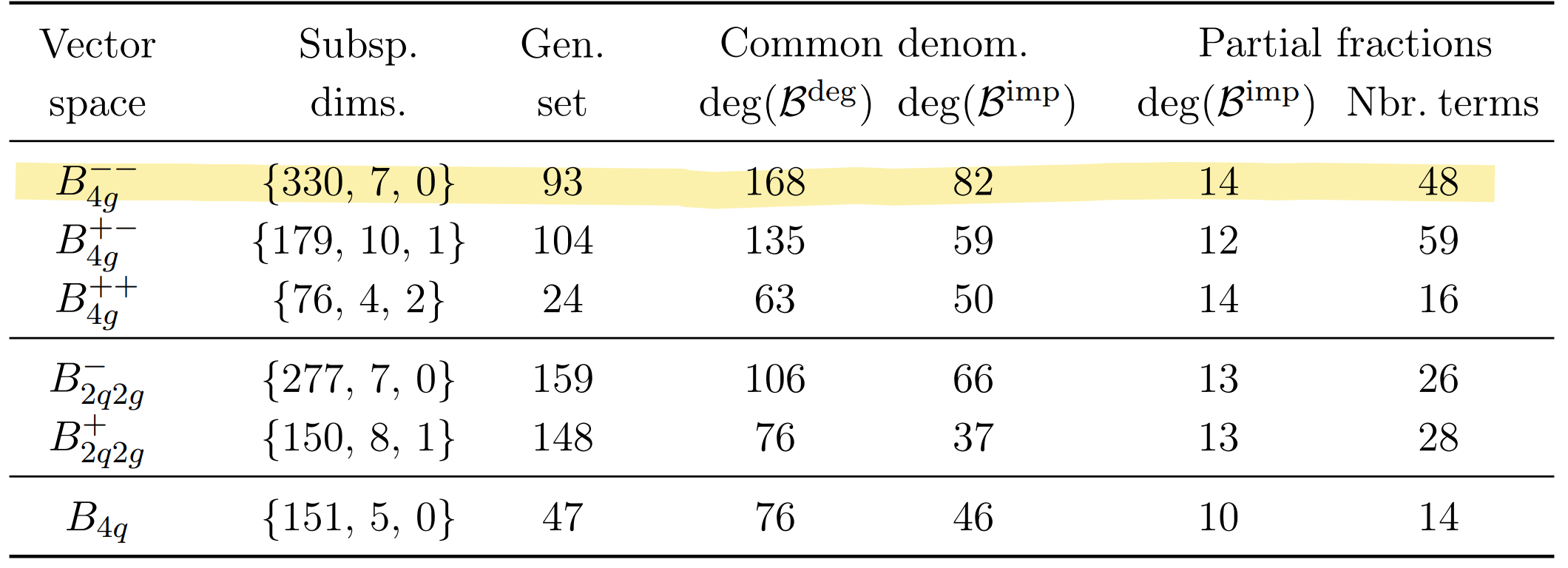
Multivariate Partial Fraction Decomposition
(Geometry beyond codimension one)
mPFD from Conjectured Properties
(for planar five-point one-mass amplitudes -- properties checked a posteriori)
$\circ\,$ Denominator pairs $\{\mathcal{D}_i, \mathcal{D}_j\}$ can be cleanly separated:
$$
\frac{\mathcal{N}}{\mathcal{D}_i^{q_i}\mathcal{D}_j^{q_j}\mathcal{D}_{\text{rest}}} \rightarrow \frac{\mathcal{N}_i}{\mathcal{D}_i^{q_i}\mathcal{D}_{\text{rest}}} + \frac{\mathcal{N}_j}{\mathcal{D}_j^{q_j}\mathcal{D}_{\text{rest}}}
$$
$\phantom{\circ}\,$ Examples of $\{\mathcal{D}_i, \mathcal{D}_j\}$ are:
$\qquad\star\,$ Any pairs of $s_{ijk}$ or $\Delta_{ij|kl|mn}$ or $\langle i|j|p_V|k|i]-\langle j|l|p_V|k|j]$
$\qquad\star\,$ Any conjugate pair $\{\langle i|j+k|l], \langle l|j+k|i]\}$ or cyclic $\{\langle i|j\rangle, [i|j]\}$
$\qquad\star\,$ Pairs of the form $\{\Delta_{ij|kl|mn}, \langle c|a+b|d] \text{ or } \langle ab \rangle \text{ or } [ab] \}$ unless $\{ab\}$ are $\{ij\}$ or $\{kl\}$ or $\{mn\}$
$\circ\,$ Other denominator pairs $\{\mathcal{D}_i, \mathcal{D}_j\}$ can be separated to order $\kappa$
$$
\frac{\mathcal{N}}{\mathcal{D}_i^{q_i}\mathcal{D}_j^{q_j}\mathcal{D}_{\text{rest}}} \rightarrow \sum_{\kappa - q_j\leq m \leq q_i}\frac{\mathcal{N}_i}{\mathcal{D}_i^{m}\mathcal{D}_j^{\kappa - m}\mathcal{D}_{\text{rest}}}
$$
$\qquad\star\,$ E.g. $\Delta_{ij|kl|mn}^4, \langle i|k+l|j]^5$ are separable to order 5.
$Vjj$ Example
$\circ\,$ Start from the function
$$
\displaystyle f^{\text{ex}} = \frac{\mathcal{N}^{\text{ex}}}{⟨14⟩^2[14]^2 s_{56} ⟨1|2+4|3]^2⟨2|1+4|3]^4⟨2|1+3|4]^2Δ_{14|23|56}^4}
$$
$\phantom{\circ}\,$ The numerator Ansatz has size 104$\,$128
$\circ\,$ Clean up the $Δ_{14|23|56}$ Gram residue
$$
\displaystyle f^{\text{ex}} = \frac{\mathcal{N}^{\text{ex}}_1}{⟨14⟩^2[14]^2s_{56}⟨2|1\!+\!4|3]^4Δ_{14|23|56}^4 \,} + \frac{\mathcal{N}^{\text{ex}}_2}{⟨14⟩^2[14]^2s_{56}⟨2|1+4|3]^4⟨1|2\!+\!4|3]^2⟨2|1\!+\!3|4]^2}
$$
$\circ\,$ Split $s_{14}$ and impose symmetry
$$
\displaystyle f^{\text{ex}} =
\frac{\mathcal{N}^{\text{ex}}_{3}}{⟨14⟩^2 s_{56} ⟨2|1+4|3]^4Δ_{14|23|56}^4}
+ \frac{\mathcal{N}^{\text{ex}}_{4}}{⟨14⟩^2 s_{56} ⟨1|2+4|3]^2⟨2|1+4|3]^4⟨2|1+3|4]^2} + (123456\rightarrow \overline{432165})
$$
$\circ\,$ Impose degree bound on poles at codimension two
$$
\displaystyle f^{\text{ex}} =
\sum_{k=0}^3 \frac{\mathcal{N}^{\text{ex}}_{5,k}}{⟨14⟩^2 s_{56} ⟨2|1+4|3]^{1+k} Δ_{14|23|56}^{4-k}}
+ \frac{\mathcal{N}^{\text{ex}}_6}{⟨14⟩^2 s_{56}⟨1|2+4|3]^2⟨2|1+4|3]^4⟨2|1+3|4]^2} + (123456\rightarrow \overline{432165})
$$
The Ansatz now has size 13$\,$532, almost a factor of 10 simpler.
mPFD as Ideal Membership
GDL, Maître ('19)
GDL, Page ('22)
$\circ$ We want a mathematically rigorous answer to the question
$$
\frac{\mathcal{N}}{\mathcal{D}_1\mathcal{D}_2} \stackrel{?}{=}
\frac{\mathcal{N}_2}{\mathcal{D}_1} + \frac{\mathcal{N}_1}{\mathcal{D}_2}
$$
$\phantom{\circ}$ without knowing $\mathcal{N}$ analytically. The complexity should not depend on $\mathcal{N}$ (besided numerical evaluations).
$\phantom{\circ}$ The complexity will depend on $\mathcal{D}_1, \mathcal{D}_2$
$\circ$ Multivariate partial fraction decompositions follow from varieties where pairs of denominator factors vanish
$$
\frac{\mathcal{N}}{\mathcal{D}_1\mathcal{D}_2} \stackrel{?}{=}
\frac{\mathcal{N}_2}{\mathcal{D}_1} + \frac{\mathcal{N}_1}{\mathcal{D}_2} \; \Longleftrightarrow \; \mathcal{N} \stackrel{?}{\in} \big\langle \mathcal{D}_1, \mathcal{D}_2 \big\rangle \, \text{ i.e. } \; \mathcal{N} \stackrel{?}{=} \mathcal{N}_1 \mathcal{D}_1 + \mathcal{N}_2 \mathcal{D}_2
$$
$$
\langle xy^2 + y^3 - z^2 \rangle + \langle x^3 + y^3 - z^2 \rangle = \langle xy^2 + y^3 - z^2, x^3 + y^3 - z^2 \rangle = \langle 2y^3-z^2, x-y \rangle \cap \langle y^3-z^2, x \rangle \cap \langle z^2, x+y \rangle
$$
$\phantom{\circ}$ This is a primary decomposition. If
$\mathcal{N}$ vanishes on all branches, than the partial fraction decomposition exists.
Challenges
$\circ\,$ How to get ideal membership information? $\mathbb{Q}_p$ points? $\mathbb{F}_p$ slice(s)?
$\circ\,$ Ideal intersection can be highly non-trivial (lcm is in general insufficient):
$$
\mathcal{N} \in \langle q_1, q_2 \rangle \cap \langle q_3, q_4 \rangle \stackrel{?}{=} \langle q_1q_3, q_1q_4, q_2q_3, q_2 q_4\rangle
$$
$\phantom{\circ}\,$ Unfortunately not always. This is called a complete intersection when it holds.
$\phantom{\circ}\,$ In general, there will be additional non-trivial generators that cannot be written in terms of $q_i$'s.
$\phantom{\circ}\,$ Therefore, either:
$\quad\star\,$ we compute the intersection explicitly (can be prohibitively hard)
$\quad\star\,$ or give up on some of the information (lose some contraining power)
$\circ\,$ Computing primary decompositions with these many variables is hard, Singular can't do it on its own.
$\phantom{\circ}\,$ Article with a Edinburgh masters' student (D. Tai) to appear. Can we avoid it? If so, at what cost?
Bivariate Slice mPFD Algorithm
$\circ$ Build a bivariate slice (curve) that intersects all varieties $V(\langle \mathcal{D}_i, \mathcal{D}_j \rangle)$, e.g.
$$
\displaystyle |i\rangle \rightarrow |i\rangle + t_1 a_i |\eta\rangle + t_2 b_i |\theta\rangle, \quad [i| \rightarrow [i| + t_1 c_i [\eta| + t_2 d_i [\theta|
$$
$\phantom{\circ}$ Such that for all $t_1, t_2$ momentum is conserved: gives 20 eqs. defining a codim.-10 variety in 24 dims
$\phantom{\circ}$ Pick sol. with syngular.Ideal.points_on_variety, impl. see lips.Particles.bivariate_slice
$\circ$ Reconstruct (Newton-interpolate) the numerators $\mathcal{N}(t_1, t_2)$; this requires $\text{deg}(\mathcal{N}+1)^2$ points.
$\circ$ For each $\mathcal{J}_{ij}^{a_i,a_j} = \big\langle \mathcal{D}_i(t_1, t_2)^{a_i}, \mathcal{D}_j(t_1, t_2)^{a_j} \big\rangle\;$ test $\;\mathcal{N}_i(t_1, t_2) \in \mathcal{J}_{ij}^{a_i,a_j}$
$\circ$ If the test passes, construct the simplified intersection from least common multiples (lcm's)
$$
\begin{equation}
\begin{aligned}\label{eq:RS_merge_generalised}
\mathcal{I}_{\rm s}'&=
\mathcal{I}_{\rm s} \cap_{s} \mathcal{J}_{ij}^{a_ia_j}:=
\big\langle
\mathrm{lcm}(m_1,n_1), \mathrm{lcm}(m_1,n_2), \ldots,
\mathrm{lcm}(m_r,n_1), \mathrm{lcm}(m_r,n_2)
\big\rangle \\
& \kern45mm \mbox{with}\quad
n_1=\mathcal{D}_i(u,v)^{a_i}
\quad\mbox{and}\quad
n_2=\mathcal{D}_j(u,v)^{a_j}\,,
\end{aligned}
\end{equation}
$$
$\phantom{\circ}$ Where $\mathcal{I}_{\rm s}$ starts as the unit ideal, and is otherwise generated by $m_1, \dots, m_r$.
$\circ$ Test $\;\mathcal{N}_i(t_1, t_2) \in \mathcal{I}_{\rm s}'$, if it passes set $\; \mathcal{I}_{\rm s} = \mathcal{I}_{\rm s}'$
Bivariate Slice mPFD Interpretation
$\circ$ In the end we are left with an ideal
$$
\begin{equation}
\mathcal{I}_{\rm s}=\langle m_1(\mathcal{D}),\ldots,m_r(\mathcal{D})\rangle \quad
\mbox{with} \quad \mathcal{N} \in \mathcal{I}_{\rm s} \,.
\end{equation}
$$
$\phantom{\circ}$ whose genreators $m_k$ are monomials in the denominator factors $\mathcal{D}_i$,
$$
\begin{align}
m_k(\mathcal{D}) = \prod_j \mathcal{D}_j^{\hat q_{jk}} \in \mathcal{I}_{\rm s} \quad\mbox{with}\quad k=1,\ldots, r
\end{align}
$$
$\phantom{\circ}$ with powers not exceeding those of the LCD, i.e. no spurious singularities by construction.
$\circ$ We interpret this back in the full multivariate setting as
$$
\mathcal{N} = \sum_{k=1}^{k_{\rm max}} \mathcal{N}_k \, m_k(\mathcal{D} ) \,
$$
$\phantom{\circ}$ and thus the (tentative) multivariate decomposition
$$
\begin{equation}
\tilde r = \frac{\mathcal{N}}{\prod_j \mathcal{D}_j^{q_j}} =
\sum_{k=1}^{r} \frac{\mathcal{N}_k }{\prod_j \mathcal{D}_j^{q_{jk}}}
\quad\mbox{with} \quad \prod_j \mathcal{D}_j^{q_{jk}} = \frac{\prod_j \mathcal{D}_j^{q_{j}}}{m_k(\mathcal{D})} \, .
\end{equation}
$$
$\circ$ Verify by fitting the ansatz. If it fails, remove some ideals from the intersection.
Invariant Quotient Rings
$\circ$ Helicity amplitudes are Lorentz invariant: minimal ansätze are build in the invariant sub-rings.
$\circ$ General construction for Lorentz-Invariant sub-rings through elimination theory
$\quad\star$ Build a ring with both covariant and invariant variables
$$
\mathbb{F}\big[ |i\rangle, [i|, \langle i j\rangle , [ij] \big]
$$
$\quad\star$ Define relations among variables (on top of existing constraints)
$$
\big\{ \langle ij \rangle - \epsilon^{\beta\alpha} \lambda_{i\alpha} \lambda_{j, \beta}, [ij] - \tilde\lambda_{i\dot\alpha} \epsilon^{\dot\alpha\dot\beta} \tilde\lambda_{j, \dot\beta} \big\}
$$
$\quad\star$ Compute a lexicographical Groebner basis with invariants > covariants
$\circ$ We obtain the following invariant rings
$$
\displaystyle \mathcal{R}_{Vjj} = \frac{\mathbb{F}\big[ \langle ij\rangle : \, 1\leq i< j\leq 6, i,j \neq 5, \; [ij] : 1\leq i< j\leq 5 \big]}{\big\langle {\textstyle \sum_{i=1}^4} [5|i]\langle i |6\rangle, 34 \text{ Schouten identities} \big\rangle}
$$
$$
\displaystyle \mathcal{R}_{ttH} = \mathbb{F}\big[ \underbrace{\langle 12\rangle, \langle \boldsymbol{3}1\rangle ... ⟨2|\boldsymbol{3}|2] ... ⟨2|\boldsymbol{3}|\boldsymbol{4}|2⟩}_{37\; \text{invariants}}
\big]\Big/ \big\langle \underbrace{⟨2|\boldsymbol{3}|2]⟨2|\boldsymbol{4}|1]-⟨2|\boldsymbol{3}|1]⟨2|\boldsymbol{4}|2]-[1|2]⟨2|\boldsymbol{3}|\boldsymbol{4}|2⟩, ...}_{\text{more than} \; 90 \; \text{generators}} \big\rangle
$$
$\phantom{\circ}$ while $R_{HHH}$ has 20 invariants, subject to 122 constraints.
The Numerator Ansatz
$\circ\,$ The numerator Ansatz takes the form (massless case)
GDL, Maître ('19)
$\displaystyle \text{Num. poly} = \sum_{\vec \alpha, \vec \beta} c_{(\vec\alpha,\vec\beta)} \prod_{j=1}^n\prod_{i=1}^{j-1} \langle ij\rangle^{\alpha_{ij}} [ij]^{\beta_{ij}}$
$\phantom{\circ}$ subject to constraints on $\vec\alpha,\vec\beta$ due to: 1) mass dimension; 2) little group; 3) linear independence.
$\circ\,$ Construct the Ansatz via the algorithm from Section 2.2 of
GDL, Page ('22)
Linear independence = irreducibility by the Gröbner basis of a specific ideal.
$\circ\,$ Efficient implementation using open-source software only
$\circ\,$ Linear systems solved w/ CUDA over $\mathbb{F}_{2^{31}-1}$ ($t_{\text{solving}} \ll t_{\text{sampling}}$) w/
linac (coming soon)
cuda_row_reduce(A, field_characteristic=primes[0], verbose=False) # A is a 2D numpy.ndarray
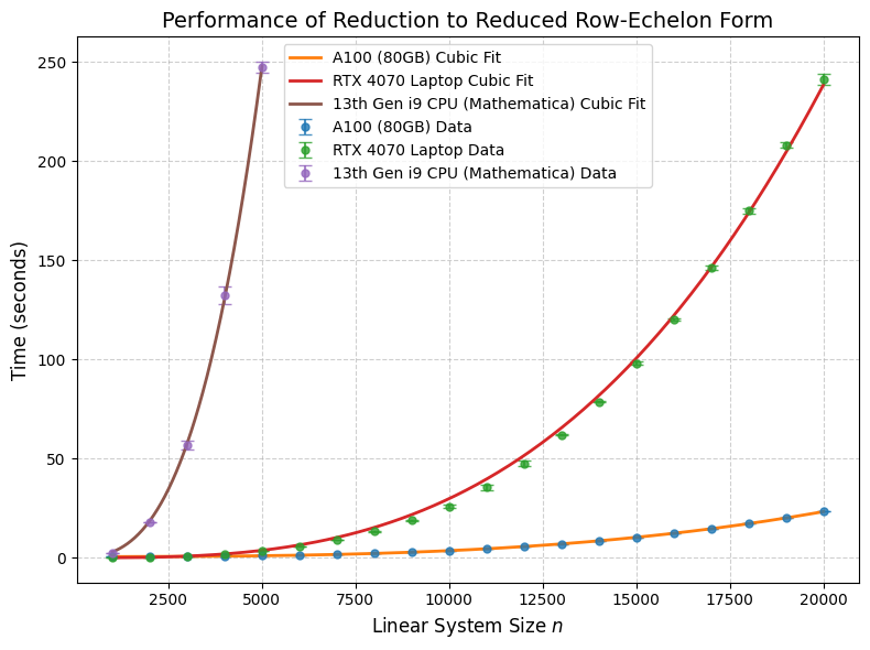
$\circ\,$ Performance on a laptop GPU of approx. 60 CPU cores
$\circ\,$ Performance on a workstation GPU of approx. 600 CPU cores
$\circ\,$ Tested on systems up to 100k equations and unknowns (takes 45 minutes).
Iterated Pole Subtraction
(i.e. geometry at codimension greater than one)
GDL, Maître ('19)
GDL, Page ('22)
Chawdhry ('23)
Xia, Yang ('25)
$\circ\,$ Iteratively reconstruct a residues at a time using $p$-adic numbers to get $\mathbb{F}_p$ samples for the residues
$$
\begin{alignedat}{2}
& r^{(139 \text{ of } 139)}_{\bar{u}^+g^+g^-d^-(V\rightarrow \ell^+ \ell^-)} = & \qquad\qquad & {\small \text{Variety (scheme?) to isolate term(s)}} \\[2mm]
& +\frac{7/4{\color{blue}(s_{24}-s_{13})}⟨6|1+4|5]s_{123}{\color{green}(s_{124}-s_{134})}}{⟨1|2+3|4]⟨2|1+4|3]^2 Δ_{14|23|56}} + & \qquad\qquad & \Big\langle ⟨2|1+4|3]^2, Δ_{14|23|56} \Big\rangle \\[1mm]
& -\frac{49/64⟨3|1+4|2]⟨6|1+4|5]s_{123}(s_{123}-s_{234})(s_{124}-s_{134})}{⟨1|2+3|4]⟨2|1+4|3]Δ^2_{14|23|56}} + \dots & \qquad\qquad & \Big\langle Δ_{14|23|56} \Big\rangle
\end{alignedat}
$$
$\circ\,$ We get more than just partial fraction decomposition, we can identify numerator insertions from e.g.:
$$
\sqrt{\big\langle ⟨2|1+4|3], Δ_{14|23|56} \big\rangle} = \big\langle {\color{green}(s_{124}-s_{134})}, ⟨2|1+4|3] \big\rangle \, , \\[1mm]
\big\langle ⟨1|2+3|4], ⟨2|1+4|3] \big\rangle = \big\langle ⟨1|2+3|4], ⟨2|1+4|3], {\color{blue}(s_{13}-s_{24})}\big\rangle \cap \big\langle ⟨12⟩, [34] \big\rangle
$$
$\circ\,$ Interesting and non-trivial bevhavior also at 5-point 3-mass
$$
\def\spa#1.#2{\left\langle#1\,#2\right\rangle}
\def\spb#1.#2{\left[#1\,#2\right]}
\def\spaa#1.#2.#3{\langle\mskip-1mu{#1}
| #2 | {#3}\mskip-1mu\rangle}
\def\spbb#1.#2.#3{[\mskip-1mu{#1}
| #2 | {#3}\mskip-1mu]}
\def\spab#1.#2.#3{\langle\mskip-1mu{#1}
| #2 | {#3}\mskip-1mu]}
\def\spba#1.#2.#3{[\mskip-1mu{#1}
| #2 | {#3}\mskip-1mu\rangle}
\def\spaba#1.#2.#3.#4{\langle\mskip-1mu{#1}
| #2 | #3 | {#4}\mskip-1mu\rangle}
\def\spbab#1.#2.#3.#4{[\mskip-1mu{#1}
| #2 | #3 | {#4}\mskip-1mu]}
\def\spabab#1.#2.#3.#4.#5{\langle\mskip-1mu{#1}
| #2 | #3 | {#4}| {#5} \mskip-1mu]}
\def\spbaba#1.#2.#3.#4.#5{[\mskip-1mu{#1}
| #2 | #3 | {#4}| {#5}\mskip-1mu\rangle}
\def\tr#1.#2{\text{tr}(#1|#2)}
\def\qb{\bar{q}}
\def\Qb{\bar{Q}}
\def\cA{{\cal A}}
\def\slsh{\rlap{$\;\!\!\not$}} \def\three{{\bf 3}}
\def\four{{\bf 4}}
\def\five{{\bf 5}}
\begin{align}\label{eq:decomp_spaba1351_spbab2542}
\big\langle \spaba1.\three.\five.1,\, \spbab2.\five.\four.2 \big\rangle = \; &\big\langle \, \spab1.\three.2,\, \spab1.\four.2,\, \spaba1.\three.\five.1,\, \spbab2.\five.\four.2
\, \big\rangle\; \cap \\
&\big\langle \, \spaba1.\three.\five.1,\, \spbab2.\five.\four.2, |\five|2]\langle1|\three| - |1+\three|2]\langle1|\five| \, \big\rangle \;, \nonumber
\end{align} \\
\text{because: } |\five|2]\spaba1.\three.\five.1[2| + |1\rangle\spbab2.\five.\four.2\langle1|\five| = \spab1.\five.2 \Big( |\five|2]\langle1|\three| - |1+\three|2]\langle1|\five| \Big) \, ,
$$
$\phantom{\circ}\,$ or between the triangle and box Grams
$$
\begin{gather}\label{eq:decomp_delta12_34_5_and_delta_12_3_4_5}
\big\langle \Delta_{12|34|5},\,\Delta_{12|3|4|5} \big\rangle =
\big\langle
s_{34},\, \tr1+2.{\three+\four}^2
\big\rangle \cap
\big\langle
\Delta_{12|34|5},\, \tr1+2.{\three-\four}^2
\big\rangle \, .
\end{gather}
$$
Iterated Pole Subtraction (another example)
$\circ$ Example from triple-Higgs
$$
\hat d^{++}_{12\times 3 \times 4}= \frac{\mathcal{N} \leftarrow 2794 \text{ free parameters }}{⟨12⟩²⟨1|𝟓|𝟒|𝟑|2]⟨2|𝟑|𝟒|𝟓|1]Δ_{12|𝟑|𝟒|𝟓}}
$$
$\circ$ We can prove $⟨1|𝟓|𝟒|𝟑|2], ⟨2|𝟑|𝟒|𝟓|1]$ can be separated, their primary decomposition reads
$$
\big\langle ⟨1|𝟓|𝟒|𝟑|2], ⟨2|𝟑|𝟒|𝟓|1] \big\rangle = \big\langle ⟨1|𝟓|𝟒|𝟑|2], ⟨2|𝟑|𝟒|𝟓|1], \text{tr}_5 \big\rangle \cap \big\langle ⟨1|𝟓|𝟒|𝟑|2], ⟨2|𝟑|𝟒|𝟓|1], s_{2𝟑}, s_{1𝟓} \big\rangle
$$
$\phantom{\circ}$ Generate two phase space points, one for each branch, and verify the numerator vanishes.
$\circ$ Similarly, with four evaluations we can prove $⟨1|𝟓|𝟒|𝟑|2], Δ_{12|𝟑|𝟒|𝟓}$ can be separated,
$$
\big\langle ⟨1|𝟓|𝟒|𝟑|2] , \, Δ_{12|𝟑|𝟒|𝟓} \big\rangle= \big\langle M_H, \; 𝟓_{\alpha\dot\alpha}𝟒^{\dot\alpha\beta} \big\rangle \cap \big\langle M_H, \; 𝟒^{\dot\alpha\alpha}𝟑_{\alpha\dot\beta} \big\rangle \cap \big\langle \langle 1 | 𝟑 | 2], \; \langle 1 | 𝟒 | 2], \; \langle 1 | 𝟑 | 𝟒 | 1 \rangle, [2 | 𝟑 | 𝟒 | 2] \big\rangle \cap \big\langle ??? \big\rangle
$$
$\phantom{\circ}$ Although we don't have a complete set of generators for the last branch, we can still sample it.
$\circ$ Fit $⟨1|𝟓|𝟒|𝟑|2]$ residue by sampling in limit $⟨1|𝟓|𝟒|𝟑|2] \rightarrow 0$
$$
\hat d^{++}_{12\times 3 \times 4} = \frac{\mathcal{N} \leftarrow 112 \text{ free parameters }}{⟨12⟩²⟨1|𝟓|𝟒|𝟑|2]} + \mathcal{O}(⟨1|𝟓|𝟒|𝟑|2]^0)
$$
Core Tools - Fully Open Source
Install from github (git clone) or PyPI (pip install); use of Jupyter is recommended.
$\circ$
pyadic
$\quad\rightarrow$ Finite field $\mathbb{F}_p$ and $p$-adic $\mathbb{Q}_p$ number types, including field extensions
$\quad\rightarrow$ rational number reconstruction (Wang's EEA, LGRR, MQRR)
$\quad\rightarrow$ univariate and multivariante Newthon & univariate Thiele interpolation algorithms in $\mathbb{F}_p$
$\circ$
syngular (in the backhand
Singular is used for many operations)
$\quad\rightarrow$ object-oriented algebraic geometry (Field, Ring, Quotient Ring, Ideal)
$\quad\rightarrow$ ring-agnostic monomials and polynomials (with support for unicode characters, e.g. spinor brackets)
$\quad\rightarrow$ multivariate solver (Ideal.point_on_variety), under- and over-constrained systems OK
$\quad\rightarrow$ a semi-numerical prime and primary ideal test (assumes equi-dimensionality of ideal)
$\circ$
lips (Lorentz invariant phase space)
$\quad\rightarrow$ phase space points over any field ($\mathbb{Q}, \mathbb{Q}[i], \mathbb{R}, \mathbb{C}, \mathbb{Q}_p, \mathbb{F}_p$), including internal and external masses
$\quad\rightarrow$ evaluate any Mandelstam or spinor expression (custom ast/regex parser)
$\quad\rightarrow$ generation of any special kinematic configuration (wrapper around Ideal.point_on_variety)
Spinor-Helicity Hjj Remainders
$\circ$ The
$pp\rightarrow Hjj$ coefficient functions are 1.5 MB of pain text LaTeX, fast and stable to evaluate.
$\phantom{\circ}$ Matrices
$M_{ij}$ account for another 22 MB. Transcendental basis at
PentagonFunctions++.
$\quad\small\rhd$ The size split is: 4gH ppmm 31%; pppm 22%, pppp 5%; 2q2gH pmpm 27%, pmpp 13%, 4qH pmpm 2%.
$\quad\small\rhd$ The largest (rational number) numerator (denominator) in the functions has 8 digits (6 digits);
$\quad\small\phantom{\rhd}$ while in the rational matrices they are 28 and 23 digits respectively.
$\quad\small\rhd$ Pheno ready results for the hard functions are available at
FivePointAmplitudes.
A Numerical CAS for Computations in Q-Rings
(partially work in progress)
$\circ$
antares (automated numerical to analytical reconstruction software)
$\rightarrow$ Univariate slicing, LCD determination, basis change, multivariate partial fractioning strategies,
$\phantom{\rightarrow}$ constraining of numerators, Ansatz generation and fitting strategies
$\rightarrow$ Limit analytic manipulations as much as possible, mostly relies on numerical evaluations.
In [1]: from antares_results.Hjj.remainders import remainder
In [2]: from antares_results.Hjj.momenta import oPs
In [3]: complex(remainder("ggggH", "pmpm_2L_Nc2_Nf0", oPs))
Out[3]: (-37.04012190864545-74.17026277643683j)
In [1]: import syngular
In [2]: from antares_results.Hjj.HTL.ggggH.ppmm import lTerms
In [3]: syngular.USE_ELLIPSIS_FOR_PRINT = True
In [4]: print(lTerms[:2], lTerms[-2:])
Out[4]: [Terms("""+(1⟨3|4⟩²)/(⟨1|2⟩²)"""), ('3412𝟓', True)] [Terms("""
+(-994/9⟨1|2⟩³⟨1|3⟩⟨2|4⟩[1|2]³+...⟪45 terms⟫...+45⟨1|2⟩⟨2|4⟩⟨3|4⟩³[2|4][3|4]²)/(⟨1|2⟩³⟨2|3⟩[2|3][3|4])
+(-45/2⟨1|2⟩⁴⟨1|3⟩²[1|2]⁶[1|3]+...⟪102 terms⟫...+45/2⟨1|2⟩⟨2|3⟩⟨3|4⟩⁴[1|3]²[2|3][2|4]³[3|4])/(⟨1|2⟩⟨1|3⟩[1|3]⟨2|3⟩[2|3][2|4][3|4]⟨2|1+3|2]²)
+(-172/3⟨1|2⟩³⟨1|4⟩[1|2]⁴[1|3][2|4]+...⟪37 terms⟫...+45/2⟨1|3⟩⟨3|4⟩³[1|2][1|3][2|3][3|4]³)/(⟨1|2⟩[1|3][2|4][3|4]⟨1|2+4|1]⟨1|2+4|3])
+(45/2⟨1|2⟩³⟨1|3⟩⟨1|4⟩²[1|2]³[1|3]+...⟪76 terms⟫...-1/3⟨1|2⟩⟨1|4⟩⟨3|4⟩⁴[2|3][3|4]³)/(⟨1|2⟩²⟨2|4⟩[3|4]⟨1|3+4|2]⟨1|2+4|3])
+⟨1|3⟩(-1/3⟨1|2⟩²⟨1|4⟩³[1|2]⁴+...⟪34 terms⟫...-1/3⟨1|4⟩⟨3|4⟩⁴[2|3]²[3|4]²)/(⟨1|2⟩⟨2|4⟩⟨1|3+4|2]²⟨1|2+4|3])
+(68/3⟨1|2⟩²⟨1|4⟩³[1|2]³[1|3]²[2|4]²+...⟪51 terms⟫...-2⟨1|4⟩⟨2|4⟩⟨3|4⟩³[1|2][2|3]²[2|4][3|4]³)/([1|3]⟨2|4⟩[2|4][3|4]⟨1|3+4|2]⟨1|2+4|3]²)
+(56/3⟨1|2⟩²⟨1|4⟩²[1|2]²[1|3][2|3][2|4]²+...⟪23 terms⟫...+8⟨1|3⟩⟨3|4⟩³[2|3]³[3|4]³)/([2|4][3|4]⟨1|2+4|3]³)
+(s_124-s_234)[1|2](2063/48⟨1|2⟩³⟨1|4⟩²[1|2]³[1|4]+...⟪84 terms⟫...-6293/72⟨1|3⟩⟨1|4⟩²⟨2|4⟩⟨3|4⟩[1|2][1|4][3|4]²)/(⟨1|2+4|3]²⟨2|1+3|4]Δ_13|24|𝟓)
+(s_124-s_234)(s_123-s_134)⟨1|3⟩²⟨2|4⟩[1|2][1|3](-23/16⟨1|2⟩⟨1|3⟩[1|2]²[1|3]+...⟪10 terms⟫...-69/16⟨2|4⟩⟨3|4⟩[1|2][2|4][3|4])/(⟨1|2+4|3]⟨2|1+3|4]Δ_13|24|𝟓²)
+[1|2](-253/2⟨1|2⟩³⟨1|3⟩⟨2|4⟩[1|2]⁴+...⟪16 terms⟫...-161/2⟨1|4⟩⁴⟨3|4⟩[1|4]⁴)/(⟨1|2+4|3]⟨2|1+3|4]Δ_13|24|𝟓)
+('2143𝟓', False, '+')
+('3412𝟓', True, '+')
+('4321𝟓', True, '+')
"""), ('1243𝟓', False)]
Effective Pentagons (another non UFD example)
$\circ$ As mentioned, pentagons can be reduced to a combination of boxes,
$$
\def\mt{m}
\def\mh{M_H}
\def\spa#1.#2{\left\langle#1\,#2\right\rangle}
\def\spb#1.#2{\left[#1\,#2\right]}
\begin{eqnarray}
&&E_0(p_1,p_2,p_3,p_4;\mt)=
c^{(1)} D_0(p_2,p_3,p_4;\mt)
+c^{(2)} D_0(p_{12},p_3,p_4;\mt) \\
&+&c^{(3)} D_0(p_1,p_{23},p_4;\mt)
+c^{(4)} D_0(p_1,p_2,p_{34};\mt)
+c^{(5)} D_0(p_1,p_2,p_3;\mt)\, .
\end{eqnarray}
$$
$\circ$ We find it useful to write the box coefficients in terms of effective pentagons $\hat e$ and boxes $\hat d$
$$
d^{h_1h_2}_{p_a\times p_b \times p_c } = \sum_{i=\{i_1,i_2\}} c^{(i)} \hat e_{p_x \times p_y \times p_z \times p_w}+ \hat d^{h_1h_2}_{p_a\times p_b \times p_c }
$$
$\phantom{\circ}$ where the sum involves the two pentagons that pinch to the given box.
$\circ$ The coefficients $\hat e$ and $\hat d$ are not uniquely defined, but $\hat e$ has the property of capturing
$\phantom{\circ}$ the residue of the poles that mix top-mass and kinematic dependence.
$\phantom{\circ}$ The non-uniqueness comes from, e.g.
$$
⟨1|2⟩[1|2]⟨1|𝟓|𝟒|𝟑|2]⟨2|𝟑|𝟒|𝟓|1]+m_t^2\text{tr}_5(1|2|𝟑|𝟒)^2=0
$$
Example of Code Syntax for Codim-2 Limit
$\circ$ This is just a couple of pip install's aways
field = Field("padic", 2 ** 31 - 1, 5)
oPs8pt = Particles(8, field=field, seed=0)
oPs8pt._singular_variety(("s_34-s_56", "s_56-s_78", '⟨1|7+8|5+6|3+4|2]', '⟨2|3+4|5+6|7+8|1]'),
                         (field.digits, field.digits, 1, 1), seed=0,
                         generators=('s_34-s_56', 's_56-s_78', '⟨1|7+8|5+6|3+4|2]',
                                     '⟨2|3+4|5+6|7+8|1]', 'tr5(1|2|3+4|5+6)'))
oPs8pt.m_t = field.random()
oPs8pt.m_h = "sqrt(s_34)"
oPs5pt = oPs.cluster([[1, ], [2, ], [3, 4], [5, 6], [7, 8]])
from antares_results.HHH.ggHHH.pp import coeffs as coeffs_pp
coeffs_pp[’d_12x3x4’](oPsC)
130808068*2147483647^-1 + 687356881 + 792807618*2147483647 + 696603492*2147483647^2 + O(2147483647^3)
The denominator goes like $p^2$, but the coefficient goes like $p^{-1} \Rightarrow$ the numerator vanishes linearly.
$\circ$ The output is a $p$-adic number, i.e. a Laurent series in powers of the prime.
$\phantom{\circ}$ With finite fields we cannot do this (with just one evaluation)! It would be dividing by zero.